Perceptron#

References-

[1]:

import numpy as np
import pandas as pd

import matplotlib.pyplot as plt
import seaborn as sns

from sklearn.datasets import make_classification

plt.style.use('seaborn')

%matplotlib inline

Algorithm Assumptions#

Binary Classification y = {-1, 1}
Data is linearly Separable

[150]:

X, y = make_classification(n_samples=50, n_features=2, n_redundant=0, n_classes=2, class_sep=2,
                           n_clusters_per_class=1, random_state=666)

y = np.where(y == 0, 1, -1) # to change classes from 0,1 to -1,1

fig = plt.figure()
ax = fig.add_subplot(1,1,1)
sns.scatterplot(x=X[:,0], y=X[:,1], hue=y, style=y, ax=ax, palette='deep')
plt.show()

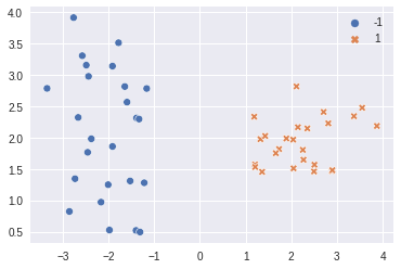
looks like data is linearly separable.

Classifier#

\(h(x_i) = sign(w^T x_i + b)\)

\begin{align*} x_i \rightarrow \begin{bmatrix} x_i \\ 1 \end{bmatrix}\\ w \rightarrow \begin{bmatrix} w \\ b \end{bmatrix} \end{align*}

if the data is shifted to center then b = 0

\(h(x_i) = sign(w^T x_i)\)

Algorithm#

Initialize \(\vec w\) = 0
While True do
- m = 0
- for \((x_i, y_i) \in D\) do
  - if \(y_i \times (w^T x_i) \le 0\) then *\(\vec{w} \leftarrow \vec{w} + y \times \vec{x}\)
    - \(m \leftarrow m + 1\)
  - end if
- end for
if m = 0 then
- break
end if
end while

\(y_i \times (w^T x_i) \gt 0\) means correctly classified sample

Implementation#

[151]:

n_samples, n_features = X.shape
w = np.zeros((n_features))

while True:
    m = 0
    for i in range(n_samples):
        if (y[i] * (w.T @ X[i])) <= 0: # misclassification
            w = w + (y[i] * X[i])
            m = m + 1

    ## if this loop was while(infinite) then when the classifier perfectly fits
    ## 0 misclassifications
    ## then m = 0 and it will break the loop
    if m == 0:
        break

[152]:

y_pred = np.int32(np.sign(w @ X.T))

[153]:

fig = plt.figure(figsize=(10,5))
ax = fig.add_subplot(1,2,1)
sns.scatterplot(x=X[:,0], y=X[:,1], hue=y, style=y, ax=ax, palette='deep')
ax.set_title("y true")

ax = fig.add_subplot(1,2,2)
sns.scatterplot(x=X[:,0], y=X[:,1], hue=y_pred, style=y_pred, ax=ax, palette='deep')
ax.set_title("y pred")

plt.show()

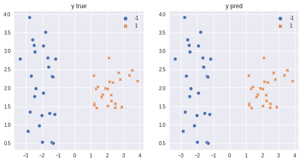
It matched most of the examples except one that is misclassified.

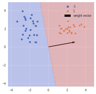
Hyperplane#

w = weight vector that defines the hyperplane

hyperplane \begin{align} \mathcal{H} = \{ x: (w^T x + b) > 0 \} \end{align} perpendicular to the weight w

[159]:

xx, yy = np.meshgrid(np.linspace(X.min() - 1, X.max() + 1, 100),np.linspace(X.min() - 1 , X.max() + 1, 100))

mesh = np.c_[xx.ravel(), yy.ravel()]
mesh_pred = np.int32(np.sign(w @ mesh.T))

zz = mesh_pred.reshape(xx.shape)

[160]:

fig = plt.figure(figsize=(5, 5))

ax = fig.add_subplot(1, 1, 1)

sns.scatterplot(x=X[:,0], y=X[:,1], hue=y, style=y, ax=ax, palette='deep')
ax.quiver(0, 0, w[0], w[1],  scale=1, units='xy',
          label='weight vector') # weight vector will always go through zero
ax.contourf(xx, yy, zz, cmap=plt.cm.coolwarm, alpha=0.3)

plt.legend()
plt.show()

Intuition#

[161]:

x = X[42,:]
origin = np.zeros_like(w)
sum_w_x = w + x

print(f"""
Origin : {origin}
x      : {x}
w      : {w}
w + x  : {sum_w_x}
""")


fig = plt.figure(figsize=(5, 5))

ax = fig.add_subplot(1, 1, 1)

ax.quiver(*origin, *x, color='b',
          scale=1, units='xy', label='data vector') # weight vector will always go through zero
ax.quiver(*w, *x, scale=1, units='xy', alpha=0.7, color='b', label='data vector')

ax.quiver(*origin, *w, color='k', scale=1,
          units='xy', label='weight vector') # weight vector will always go through zero
ax.quiver(*origin, *sum_w_x, scale=1, units='xy', color='r')
ax.contourf(xx, yy, zz, cmap=plt.cm.coolwarm, alpha=0.4)

ax.text(*x, 'x', color='b')
ax.text(*w, 'w', color='k')
ax.text(*sum_w_x, 'w + x', color='r')

plt.legend()
plt.show()


Origin : [0. 0.]
x      : [-2.73210556  1.34370036]
w      : [2.95108238 0.53659625]
w + x  : [0.21897682 1.8802966 ]

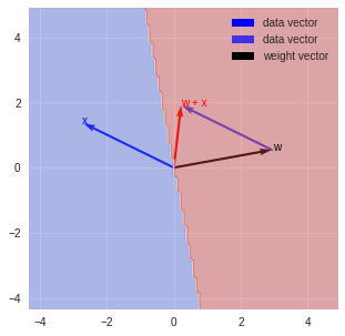
\begin{align} \vec{w} x \le 0\\ \text{ after k updates/iterations } (w + kx)^T x \le 0 \\ \text{ and still getting it wrong}\\ w^Tx + k x^Tx \le 0\\ k \le \frac{- w^Tx}{x^Tx} \end{align}

this explains that k exists as a solution less than infinite.

\begin{align} \text{there exists } \exists{w^*} && s.t. \forall(\vec{x},\vec{y}) \in D && yw^Tx \gt 0\\ ||w^*|| = 1\\ ||\vec{x}|| \lt 1 && \forall (\vec{x},\vec{y}) \in D\\ \\ yw^Tx \gt 0 \begin{cases} y = +1 \Rightarrow w^Tx \gt 0\\ y = -1 \Rightarrow w^Tx \lt 0\\ \end{cases}\\ \\ w \leftarrow w + yx \begin{cases} y = +1 \Rightarrow w \leftarrow w + x\\ y = -1 \Rightarrow w \leftarrow w - x\\ \end{cases} \end{align}

\(w^*\) is the optimum solution.

Margin#

Minimum distance from closest data poin and hyperplane.

\begin{align} \gamma = {min\atop{x,y \in D}} | x^T w^* | \gt 0 \end{align}

[165]:

distances = np.abs(w @ X.T)
min_dist_idx = np.argmin(distances)

print(f"""
minimum distance index : {min_dist_idx}
gamma                  : {distances[min_dist_idx]}
""")

fig = plt.figure(figsize=(10, 5))

ax = fig.add_subplot(1, 2, 1)

sns.scatterplot(x=X[:,0], y=X[:,1], hue=y, style=y, ax=ax, palette='deep')
ax.contourf(xx, yy, zz, cmap=plt.cm.coolwarm, alpha=0.3)

ax = fig.add_subplot(1, 2, 2)

sns.scatterplot(x=X[:,0], y=X[:,1], hue=y, style=y, ax=ax, palette='deep')
ax.contourf(xx, yy, zz, cmap=plt.cm.coolwarm, alpha=0.3)
sns.scatterplot(x=X[min_dist_idx,[0]], y=X[min_dist_idx,[1]], color='k',
                marker='o', ax=ax, label='min distant point')

plt.legend()
plt.show()


minimum distance index : 49
gamma                  : 1.94312938664885

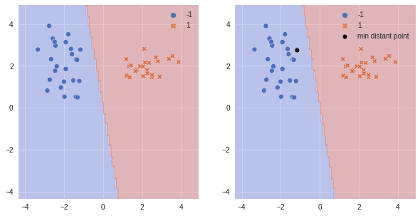
typically we want a large margin classifier.(we will go back to svm for this)

with each iteration atleast a gamma is added.

\begin{align} w^Tw^* + y(x^T w^*) \ge w^Tw^* + \gamma \end{align}

Perceptron

Contents