Bias-Variance Tradeoff

Reference

• https://www.youtube.com/watch?v=pvcEQfcO3pk (stanford youtube)

• ISLR

Concept

• Bias-Variance Tradeoff is a fundamental concept of Machine Learning to address challenges of model performance and generalization.

\begin{align*} Err(x) = Bias^2 + Variance + irreducible \end{align*}

There are 2 concepts in Bias-Variance Tradeoff

Bias Error

• Bias is explained by inabilty to capture the true relationship between dependent and independent variable.

• It means approximation of real world problem with a generalized/simple model

• High bias means model made significant assumptions about data that it doesn’t actually learn the underlying pattern or complexity of real world data.

• In essence model was too simple that it couldn’t learn the pattern and resulted in underfitting. This model will perform poorly on both training data as well as testing data

Variance Error

• differene in model fit and actual values of the dataset.

• High Variance means that the model is flexible(complex) and fits training data closely (even captures random fluctuations)

• The amount at which model fit will change it we change the training data, If a method has high variance then a small change in training data can result in large change in model fit.

• In essence model was too complex that it learnt every possible pattern and resulted in overfitting. This model will perform well on training data but can perform poorly on testing or on real world data.

Data Prep

import pandas as pd
import numpy as np
from sklearn.datasets import make_regression, load_diabetes
from sklearn.model_selection import train_test_split
import matplotlib.pyplot as plt

plt.style.use('fivethirtyeight')

sample_size = 200
train_size = 0.65
random_state = 5000
np.random.seed(random_state)

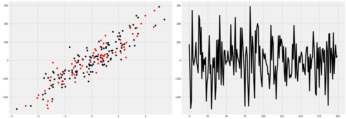
X, y = make_regression(n_samples=sample_size, n_features=1, n_informative=1, noise=45, random_state=random_state, shuffle=True)

X_train, X_test, y_train, y_test = train_test_split(X, y, train_size=train_size, random_state=random_state)

fig, ax = plt.subplots(1, 2, figsize=(20, 7))

ax[0].plot(X_train, y_train, 'ko')
ax[0].plot(X_test, y_test, 'ro')

ax[1].plot(y, 'k.-')

plt.tight_layout()
plt.show()

Proof

using polynomial regression with increasing number of degrees for simple to complex(more flexible) model.

from sklearn.linear_model import LinearRegression
from sklearn.preprocessing import PolynomialFeatures
from sklearn.metrics import mean_squared_error
from sklearn.pipeline import make_pipeline

def model_performance(X_train, X_test, y_train, y_test, poly_degree):

    model = make_pipeline(PolynomialFeatures(degree=poly_degree, include_bias=False), LinearRegression())
    model.fit(X_train, y_train)
    y_train_hat = model.predict(X_train)
    y_test_hat = model.predict(X_test)

    mse_train = mean_squared_error(y_train, y_train_hat)
    mse_test = mean_squared_error(y_test, y_test_hat)

    return None, mse_train, mse_test

mse_train_list = []
mse_test_list = []
poly_degrees = [1, 2, 3, 4, 5, 6, 7, 8, 9, 10, 11, 12, 13, 14, 15]

for degree in poly_degrees:
    _, mse_train, mse_test = model_performance(X_train, X_test, y_train, y_test, degree)
    mse_train_list.append(mse_train)
    mse_test_list.append(mse_test)

def moving_average(a, n=3):
    ret = np.cumsum(a, dtype=float)
    ret[n:] = ret[n:] - ret[:-n]
    return ret[n - 1:] / n

fig, ax = plt.subplots(1, 1, figsize=(7, 7))

ax.plot(moving_average(mse_train_list, n=5)[:-2], 'o-', label='rolling mean train mse')
ax.plot(moving_average(mse_test_list, n=5)[:-2], 'o-', label='rolling mean test mse')

ax.set_xlabel('flexibility')
ax.set_ylabel('MSE')

plt.suptitle("Bias-Variance Tradeoff")
plt.legend()
plt.show()

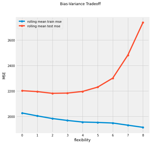
• On left side, the model is really simple(degree 1 polynomial regression), shows high bias, performed poor on both train and test data.

• On right side, the model is more flexible(high degree polynomial regression), shows high variance, performed well on training data(low mse), but performed poorly on test data.