
Fourier Transform#
[1]:
import math
import numpy as np
import matplotlib.pyplot as plt
from matplotlib import style
from IPython import display
from matplotlib import animation


style.use('ggplot')

# %matplotlib inline
Euler’s Number(e)#
[2]:
math.e,np.e
[2]:
(2.718281828459045, 2.718281828459045)
[3]:
plt.plot(np.exp(np.arange(-10,30,0.1)))
[3]:
[<matplotlib.lines.Line2D at 0x7f5b54eb8670>]

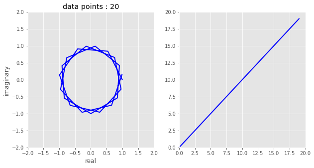
\(e^{\pi i}\)#
[4]:
N = 20
fig = plt.figure(figsize=(10,5))
ax1 = plt.subplot(1,2,1)
ax2 = plt.subplot(1,2,2)

ax1.set_xlim((-2, 2))
ax1.set_ylim((-2, 2))
ax1.set_xlabel("real")
ax1.set_ylabel("imaginary")

ax2.set_xlim((0,N))
ax2.set_ylim((0,N))


txt_title = ax1.set_title('data points : 0')
plot1, = ax1.plot([], [], 'b-', lw=2)
plot2, = ax2.plot([], [], 'b-', lw=2)

def draw_frame(n):
    a = np.arange(n+1)
    data = np.exp(1j * a)
    plot1.set_data(data.real,data.imag)
    plot2.set_data(range(n+1),a)
    txt_title.set_text(f"data points : {n+1}")
    return (plot1,)

anim = animation.FuncAnimation(fig, draw_frame, frames=N, interval=1000, blit=True)

display.HTML(anim.to_html5_video())
[4]:
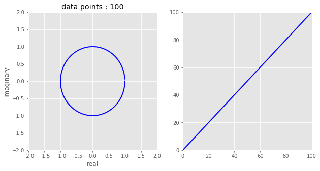
\(e^{-2\pi\frac{i}{N}}\)#
[5]:
N = 100
fig = plt.figure(figsize=(10,5))
ax1 = plt.subplot(1,2,1)
ax2 = plt.subplot(1,2,2)

ax1.set_xlim((-2, 2))
ax1.set_ylim((-2, 2))
ax1.set_xlabel("real")
ax1.set_ylabel("imaginary")

ax2.set_xlim((0,N))
ax2.set_ylim((0,N))


txt_title = ax1.set_title('data points : 0')
plot1, = ax1.plot([], [], 'b-', lw=2)
plot2, = ax2.plot([], [], 'b-', lw=2)

def draw_frame(n):
    a = np.arange(n+1)
    data = np.exp(-2j * np.pi * a/N)
    plot1.set_data(data.real,data.imag)
    plot2.set_data(range(n+1),a)
    txt_title.set_text(f"data points : {n+1}")
    return (plot1,)

anim = animation.FuncAnimation(fig, draw_frame, frames=N, interval=100, blit=True)

display.HTML(anim.to_html5_video())
[5]:
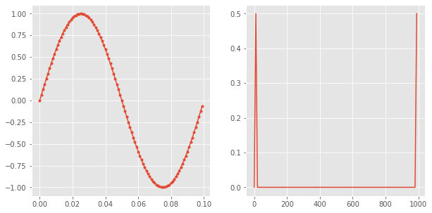
Sine wave#
\(A_{shift} + A \sin(2{\pi}{f}{t} + \phi )\)
[6]:
np.linspace(0,10,5) # evenly spaced 5 numbers between 0 to 10
[6]:
array([ 0. , 2.5, 5. , 7.5, 10. ])
[7]:
def sine_wave(n_samples, signal_freq, n_cycles = 10, amplitude = 1, amp_shift = 0, phase_shift = 0):
    """Sine wave generation
    """
    sampling_freq = (n_samples * signal_freq) / n_cycles
    # n_samples = int((sampling_freq / signal_freq) * n_cycles)

    t_step = 1 / sampling_freq
    time = np.linspace(0, (n_samples-1) * t_step , n_samples)

    f_step = sampling_freq / n_samples
    freq = np.linspace(0, (n_samples-1) * f_step , n_samples)

    wave = amp_shift + amplitude * np.sin( (2 * np.pi * signal_freq * time) + phase_shift)

    return wave, time, freq
[8]:
N = 100
wave, time, freq = sine_wave(
    n_samples = N,
    signal_freq = 10,
    n_cycles = 1,
    amplitude = 1,
    amp_shift = 0,
    phase_shift = 0
)

fig,ax = plt.subplots(1,2,figsize=(10,5))

ax[0].plot(time,wave,".-")
ax[1].plot(freq,np.abs(np.fft.fft(wave))/N)

plt.show()
[9]:
fig = plt.figure(figsize=(16,8))
ax = fig.add_subplot(111)


wave, time, _ = sine_wave(
    n_samples = 50,
    signal_freq = 10,
    n_cycles = 5
)
ax.plot(time, wave, 'r-*')

wave, time, _  = sine_wave(
    n_samples = 40,
    signal_freq = 10,
    n_cycles = 5
)
ax.plot(time, wave, 'b-*')

wave, time, _  = sine_wave(
    n_samples = 30,
    signal_freq = 10,
    n_cycles = 5
)
ax.plot(time, wave, 'g-*')


wave, time, _  = sine_wave(
    n_samples = 10,
    signal_freq = 10,
    n_cycles = 5
)
ax.plot(time, wave, 'c-*')

plt.show()

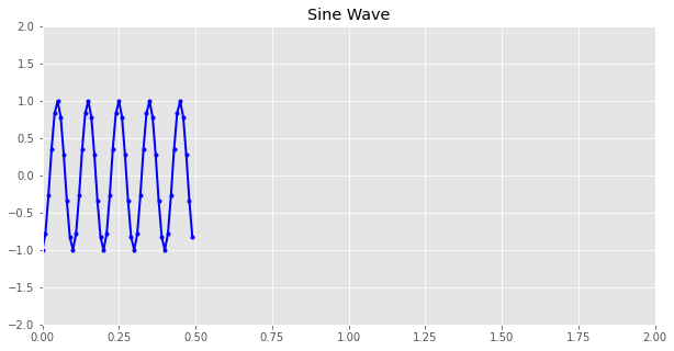
Sine Wave Animation#
[10]:
fig = plt.figure(figsize=(10,5))
ax1 = plt.subplot(1,2,(1,2))

ax1.set_xlim(( 0, 2))
ax1.set_ylim((-2, 2))

txt_title = ax1.set_title('Sine Wave')
plot1, = ax1.plot([], [], 'b.-', lw=2)

def draw_frame(n):
    wave, time, _  = sine_wave(
        n_samples = 50,
        signal_freq = 10,
        n_cycles = 5,
        phase_shift=n
    )
    plot1.set_data(time,wave)
    return (plot1,)

anim = animation.FuncAnimation(fig, draw_frame, frames=100, interval=100, blit=True)

display.HTML(anim.to_html5_video())
[10]:
Discrete Fourier Transform#
\(X_{k} = \sum_{n=0}^{N-1} x_n e^{-{i}{2}{\pi}{k}\frac{n}{N}}\)
Discrete fourier transform with iteration#
[11]:
def freq_plane(x,k,N):
    return x * np.exp(-1j *2 * np.pi * k * (np.arange(N)/N))

def fourier_transform_old(x):
    N = x.shape[0]
    values = []
    for k in range(N):
        X_k = (freq_plane(x,k,N)).sum()
        values.append(X_k)

    X = np.array(values)
    return X
but this is not optimized way to calculate.
I learnt this new method to use matrix multiplication and broadcasting in machine learning gradient descent calculation
Optimized discrete fourier transform#
expanding the submission.. and looking for patterns to multiply \begin{align} X_0 &= e^\frac{i2\pi}{N}[ x_0 e^{0.0} + x_1 e^{0.1} + \dots + x_{N-1} e^{0.N-1} ]\\ X_1 &= e^\frac{i2\pi}{N}[ x_0 e^{1.0} + x_1 e^{1.1} + \dots + x_{N-1} e^{1.N-1} ]\\ \dots \\ X_{N-1} &= e^\frac{i2\pi}{N}[ x_0 e^{{N-1}.0} + x_1 e^{{N-1}.1} + ... + x_{N-1} e^{{N-1}{N-1}} ] \end{align}
Transforming in matrix
\(\begin{bmatrix} X_{0} & X_{1} \dots & X_{N-1} \end{bmatrix} = \\ \begin{bmatrix} x_{0} & x_{1} \dots & x_{N-1} \end{bmatrix} * e^{\frac{i2\pi}{N}} \begin{bmatrix} e^{0.0} & e^{0.1} & e^{0.2} & \dots & e^{0.N-1} \\ e^{1.0} & e^{1.1} & e^{1.2} & \dots & e^{1.N-1} \\ \dots \\ e^{N-1.0} & e^{N-1.1} & e^{N-1.2} & \dots & e^{N-1.N-1} \end{bmatrix}\)
Preparing \(k \times n\)
\begin{align} k &= \begin{bmatrix} k_0 \\ k_1 \\ k_2 \\ \dots \\ k_N-1 \end{bmatrix} \\ n &= \begin{bmatrix} n_0 & n_1 & n_2 & \dots & n_N-1 \end{bmatrix}\\ \text{Broadcasting }\\ \\ k \times n &= \begin{bmatrix} k_0.n_0 & k_0.n_1 & \dots & k_0.n_{N-1} \\ k_1.n_0 & k_1.n_1 & \dots & k_1.n_{N-1} \\ \dots \\ k_{N-1}.n_0 & k_{N-1}.n_1 & \dots & k_{N-1}.n_{N-1} \\ \end{bmatrix} \end{align}
[12]:
def fourier_transform(x):
    """Discrete Fourier Transform (DFT).

    Notes:
        This is faster and optimized approach.
        using numpy matrix multiplication here.
    """

    N = x.shape[0]
    n = np.arange(N) # an array of size N-1
    k = n.reshape(-1,1) # freq idxs with (N-1,1)


    # with numpy broadcasting
    # k (N-1,1) is broadcasted over n (N-1,) and result is
    m_value = np.exp(-2 * np.pi * k * (n/N) * 1j)
    # (N-1,N-1)

    X = x @ m_value
    # (N-1,) * (N-1,N-1)
    # actually it is broadcasting
    return X
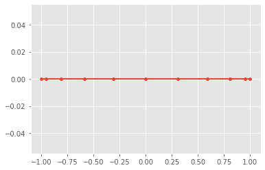
Winding plane#
here we are using an iterative approach to do the transform. because we want each plane for ever frequency to visualize
[13]:
N = 100
wave, time, freqs  = sine_wave(
    n_samples = N,
    signal_freq = 50,
    n_cycles = 5
)
[14]:
plane = freq_plane(wave,0,N)
plt.plot(plane.real,plane.imag,'.-')
plt.show()
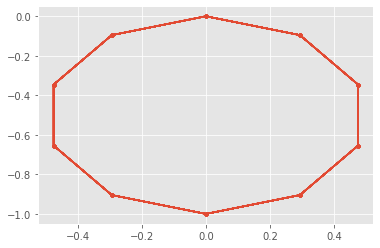
[15]:
plane = freq_plane(wave,1,N)
plt.plot(plane.real,plane.imag,'.-')
plt.show()
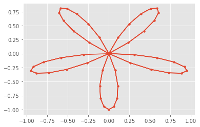
[16]:
plane = freq_plane(wave,5,N)
plt.plot(plane.real,plane.imag,'.-')
plt.show()
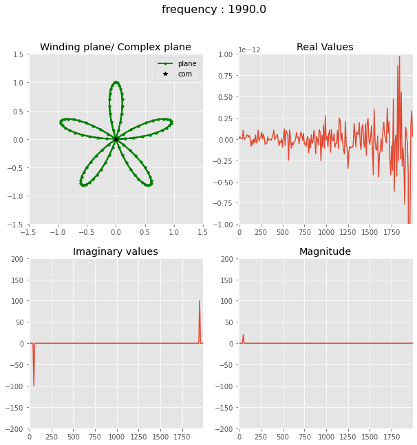
[17]:
N = 200
wave, time, freqs  = sine_wave(
    n_samples = N,
    signal_freq = 50,
    n_cycles = 5
)


fig = plt.figure(figsize=(10,10))
ax1 = plt.subplot(2,2,1)
ax2 = plt.subplot(2,2,2)
ax3 = plt.subplot(2,2,3)
ax4 = plt.subplot(2,2,4)

ax1.set_xlim((-1.5, 1.5))
ax1.set_ylim((-1.5, 1.5))

ax2.set_xlim((-10, freqs[-1]))
ax2.set_ylim((-1e-12, 1e-12))

ax3.set_xlim((-10, freqs[-1]))
ax3.set_ylim((-200, 200))

ax4.set_xlim((-10, freqs[-1]))
ax4.set_ylim((-200, 200))

txt_title = fig.suptitle('This is a somewhat long figure title', fontsize=16)
ax1.set_title('Winding plane/ Complex plane')
ax2.set_title('Real Values')
ax3.set_title('Imaginary values')
ax4.set_title('Magnitude')
plot1, = ax1.plot([], [], 'g.-', lw=2, label='plane')
plot2, = ax1.plot([], [], 'k*', label='com')
plot3, = ax2.plot([], [])
plot4, = ax3.plot([], [])
plot5, = ax4.plot([], [])

ax1.legend()


real_com = []
imag_com = []
coms = []
i_com = []

def draw_frame(n):
    plane = freq_plane(wave,n,N)
    com = plane.sum()
    real_com.append(com.real)
    imag_com.append(com.imag)
    coms.append(abs(com)/n)
    i_com.append(freqs[n])

    plot1.set_data(plane.real,plane.imag)
    plot2.set_data(com.real,com.imag)
    plot3.set_data(i_com,real_com)
    plot4.set_data(i_com,imag_com)
    plot5.set_data(i_com,coms)
    txt_title.set_text(f"frequency : {freqs[n]}")
    return (plot1,plot2,plot3,plot4,plot5)

anim = animation.FuncAnimation(fig, draw_frame, frames=N, interval=1000, blit=True)

display.HTML(anim.to_html5_video())
<ipython-input-17-358f6cd05818>:51: RuntimeWarning: divide by zero encountered in double_scalars
  coms.append(abs(com)/n)
<ipython-input-17-358f6cd05818>:51: RuntimeWarning: divide by zero encountered in double_scalars
  coms.append(abs(com)/n)
[17]:
Symmetries in DFT#
\begin{align} X_{k} &= \sum_{n=0}^{N-1} x_n e^{-{i}{2}{\pi}{k}\frac{n}{N}}\\ X_{N+k} &= \sum_{n=0}^{N-1} x_n e^{-{i}{2}{\pi}{(N+k)}\frac{n}{N}}\\ X_{N+k} &= \sum_{n=0}^{N-1} x_n e^{-{i}{2}{\pi}{N}} e^{-{i}{2}{\pi}{k}\frac{n}{N}}\\ e^{-{i}{2}{\pi}{N}} &= 1\\ X_{N+k} &= \sum_{n=0}^{N-1} x_n e^{-{i}{2}{\pi}{k}\frac{n}{N}}\\ X_{N+k} &= X_k\\ X_{k + i.N0} &= X_k \end{align}
Cooley and Tukey used exactly this approach in deriving the Fast Fourier Transform.
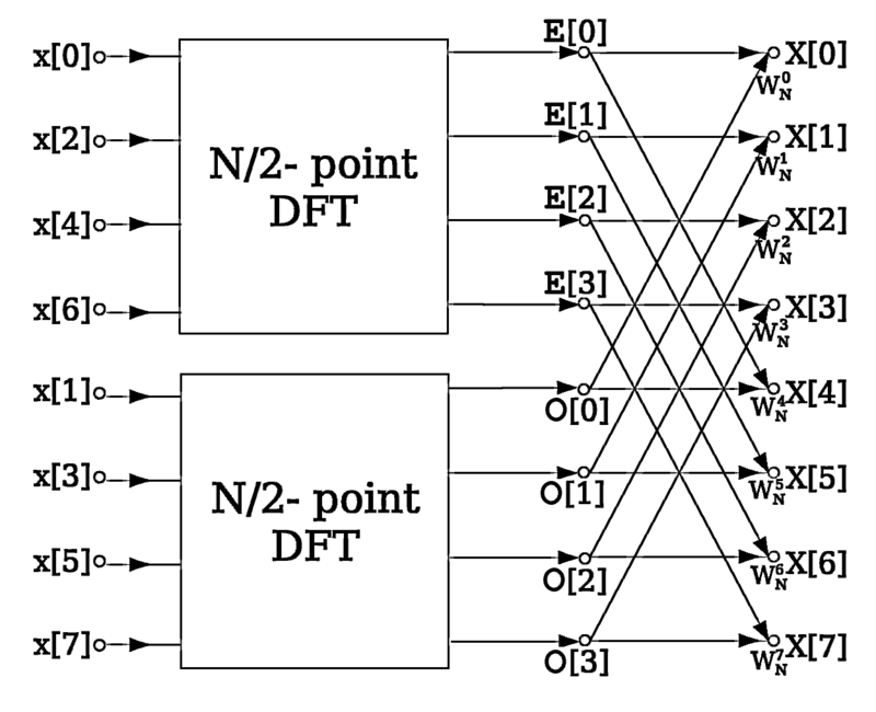
Fast Fourier Transform#
concept for odd and even numbers\begin{align} X_{k} &= \sum_{n=0}^{N-1} x_n e^{-{i}{2}{\pi}{k}\frac{n}{N}}\\ X_{k} &= \sum_{m=0}^{(N/2)-1} x_{2m} e^{-{i}{2}{\pi}{k}\frac{2m}{N}} + \sum_{m=0}^{(N/2)-1} x_{2m+1} e^{-{i}{2}{\pi}{k}\frac{2m+1}{N}}\\ X_{k} &= \sum_{m=0}^{(N/2)-1} x_{2m} e^{-{i}{2}{\pi}{k}\frac{2m}{N}} + e^{-{i}{2}{\pi}{\frac{k}{N}}} \sum_{m=0}^{(N/2)-1} x_{2m+1} e^{-{i}{2}{\pi}{k}\frac{2m}{N}}\\ X_{k} &= \sum_{m=0}^{(N/2)-1} x_{2m} e^{-{i}{2}{\pi}{k}\frac{m}{N/2}} + e^{-{i}{2}{\pi}{\frac{k}{N}}} \sum_{m=0}^{(N/2)-1} x_{2m+1} e^{-{i}{2}{\pi}{k}\frac{m}{N/2}} \end{align}
FFT algorithm#
[18]:
np.array([0,1,2,3,4,5])[::2] # numpy selecting even indices
[18]:
array([0, 2, 4])
[19]:
np.array([0,1,2,3,4,5])[1::2] # numpy selecting odd indices
[19]:
array([1, 3, 5])
[20]:
np.concatenate(
    [
        np.array([0,1,2,3,4,5])[::2],
        np.array([0,1,2,3,4,5])[1::2]
    ]
)
[20]:
array([0, 2, 4, 1, 3, 5])
[21]:
def fast_fourier_transform(x):
    """Fast Fourier Transform.
    """
    N = x.shape[0]
    if np.log2(N) % 1 > 0:
        raise ValueError("""
        Length of the signal is not in the power of 2. Padding will be required.
        """)
    elif N <= 32: #we need a minimum threshold after that the slow transformation is calculated
        return fourier_transform(x)

    else:
        X_even = fast_fourier_transform(x[::2])
        X_odd = fast_fourier_transform(x[1::2])

        k = np.arange(N)

        m_factor = np.exp(-2j * np.pi * (k/N))
        break_point = int(N/2) # we need a break point to break the factors in half
        # as the enen and odd arrays are size of N/2
        # otherwise mulitiplication cant happen

        t = np.concatenate(
            [
                X_even + m_factor[:break_point] * X_odd,
                X_even + m_factor[break_point:] * X_odd
            ]
        )
        return t
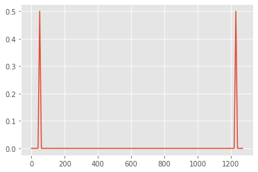
[22]:
N = 128
wave, time, freqs  = sine_wave(
    n_samples = N,
    signal_freq = 50,
    n_cycles = 5
)
result = fast_fourier_transform(wave)
[23]:
plt.plot(freqs,np.abs(result)/N)
[23]:
[<matplotlib.lines.Line2D at 0x7f5b4cce7fa0>]

Inverse Frequency Fourier Transform#
\(x_{k} = \frac{1}{N}\sum_{n=0}^{N-1} X_n e^{{i}{2}{\pi}{k}\frac{n}{N}}\)
[24]:
def inv_fourier_transform(X):
    N = X.shape[0]
    n = np.arange(N) # an array of size N-1
    k = n.reshape(-1,1) # freq idxs with (N-1,1)

    # with numpy broadcasting
    # k (N-1,1) is broadcasted over n (N-1,) and result is
    m_value = np.exp(2 * np.pi * k * (n/N) * 1j)
    # (N-1,N-1)

    x = X @ m_value
    # (N-1,) * (N-1,N-1)
    # actually it is broadcasting

    return x/N
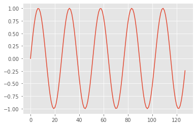
[25]:
N = 128
wave, time, freqs  = sine_wave(
    n_samples = N,
    signal_freq = 50,
    n_cycles = 5
)

plt.plot(wave)
[25]:
[<matplotlib.lines.Line2D at 0x7f5b4cd74b80>]
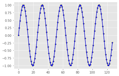
[26]:
dft_values = fast_fourier_transform(wave)
[27]:
inv_values = inv_fourier_transform(dft_values)

plt.plot(inv_values.real,'y*-')
plt.plot(wave,'b.-')
[27]:
[<matplotlib.lines.Line2D at 0x7f5b4cced7f0>]
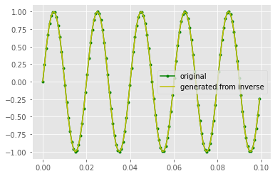
Using numpy fft methods#
[28]:
N = 128
wave, time, freqs  = sine_wave(
    n_samples = N,
    signal_freq = 50,
    n_cycles = 5
)
[29]:
f_v = np.fft.fft(wave)
mag_f_v = np.abs(f_v) / N
plt.plot(freqs,mag_f_v)
[29]:
[<matplotlib.lines.Line2D at 0x7f5b4ccc0fa0>]
[30]:
i_v = np.fft.ifft(f_v)

plt.plot(time,wave,'g.-',label="original")
plt.plot(time,i_v.real,'y-',label='generated from inverse')
plt.legend()
plt.show()
[31]:
%timeit fourier_transform(wave)
5.61 ms ± 298 µs per loop (mean ± std. dev. of 7 runs, 100 loops each)
[32]:
%timeit np.fft.fft(wave)
7.2 µs ± 149 ns per loop (mean ± std. dev. of 7 runs, 100000 loops each)
[33]:
%timeit fast_fourier_transform(wave)
1.24 ms ± 27.3 µs per loop (mean ± std. dev. of 7 runs, 1000 loops each)