
Experiments & Testing#
References#
The ASA Statement on p-Values: Context, Process, and Purpose
https://en.wikipedia.org/wiki/Student%27s_t-test#Dependent_t-test_for_paired_samples
[1]:
import numpy as np
import pandas as pd
import matplotlib.pyplot as plt
import seaborn as sns
                 Start
                   |
                   v
          Formulate Hypothesises
                   |
                   v
Formulate analysis plan and Design Experiment
                   |
                   v
              Analyze data
                   |
                   v
           Interpret Results
                   |
                   v
                  End
A/B test#
Treatment activity in which drug, price, etc. exposed to a subject.
Subjects participants in treatment.
Treatment Group group of subjects exposed to treatment.
Control Group group of subjects not exposed to treatment.
Randomization randomly selecting subjects to put in groups.
test statistics the metric used to measure the effect of the treatment.
In A/B test an experiment is established, two groups for a treatment, one group will follow up on existing/standard treatment or no treatment called Control group, and the other one will follow up on new treatment called Treatment Group
Generally the difference between the groups
The effect of the different treatments.
because of randomness, by luck subjects are assigned to which group for results to perform better.(or better performing subjects concentrated in A or B)
So now what test statistics or metrics to compare groups A or B. Most common is binary.(buy or not-buy, click or not-clicked, fraud or no-fraud)
I am gonna take a very non-medical example to understand this. So there are two advertisements(types of ads) on a website and we are trying to test with group of people, randomly 90 people selected for ad A and randomly 90 people selected for ad B , whether they will click or not click on the ad.
so we have this kind of metrics as result of the experiment.
         |
Outcome  |   Advert A     Advert B
_________|__________________________
click    |
         |
no-click |
[2]:
actions = np.array(['no-click','click'])
[3]:
np.random.seed(0)

group_A = np.random.choice(actions,size=90, p=[0.4,0.6]) # have to give some bias to generate some sided choices
group_B = np.random.choice(actions,size=90, p=[0.2,0.8])

df = pd.DataFrame()
df['Advert A'] = group_A
df['Advert B'] = group_B

df.head()
[3]:
| Advert A | Advert B | |
|---|---|---|
| 0 | click | click |
| 1 | click | click |
| 2 | click | no-click |
| 3 | click | click |
| 4 | click | click |
[4]:
result_df = pd.DataFrame()

result_df['Advert A'] = df['Advert A'].value_counts()
result_df['Advert B'] = df['Advert B'].value_counts()

result_df
[4]:
| Advert A | Advert B | |
|---|---|---|
| click | 55 | 73 |
| no-click | 35 | 17 |
[5]:
fig, ax = plt.subplots(1,2,figsize=(10,5))

ax[0].hist(df['Advert A'],color='g')
ax[0].set_title('Advert A')
ax[0].set_ylim((0,90))

ax[1].hist(df['Advert B'],color='c')
ax[1].set_title('Advert B')
ax[1].set_ylim((0,90))

plt.show()
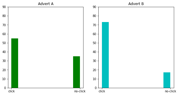
normally as a data scientist the question I have in my mind while using A/B testing that which ad performed better?
Metrics#
Success Metric/ Goal Metric#
(North Start, OKR, Primary)
Company mission & visions are measured from this
Simple to communicate with stakeholders
Stable over long period of time
May not be suitable for online experiments
Difficult to measure
Not sensitive to product changes
eg.- Revenue
Driver Metric#
(Surrogate, Indirect/Predictive)
Short term objective
Align with Goal Metrics
More sensitive and actionable
Better for A/B testing
eg.- User acquisition
success metrics \(\ne\) driver metrics
Success Metrics |
Driver Metrics |
|---|---|
long term |
short term, suitable for experimentation |
Guardrail Metric#
Guard business from
Harming business
Violating assumptions
Organisational Guardrail Metrics > Negative -> Business will suffer significant loss
loading time of home page -> drop in user count -> loss in revenue
page loading latency, crashes etc.
Trustworthy-related Metrics > Check trustworthyness of experiments > Check violations and assumptions > eg.- Randomization units assigned to variants
Hypothesis Test/ Significance Test#
The purpose is to learn whether random chance might be responsible for an observed effect
Test Statisitcs#
Metric for difference or effect of interest from test.
Null Hypothesis (\(H_0\))#
The hypothesis that chance is to blame.
To check whether claim is applicable or not
States that there is no significant difference between a set of a variable
in simple words everything is same or equal
By why do we need this? So lets say for A/B tseting we have randomly selected people for control and treatment group. After introducing randomness in the experiment it is okay to assume that any similarity in the groups is completely by chance. But to idenitify this similarity between groups we need a baseline assumption that there is a similarity/ equivalency to be measured. This baseline assumption is Null hypothesis(eg. both of the groups have equal mean height.\(\mu_1 = \mu_2\)). And to clarify that there is no similarity Null Hypothesis has to be rejected with test statisitcs.
Alternate Hypothesis (\(H_1\) / \(H_a\))#
to challenge currently accepted state of knowledge
more precisely states that there is a significant difference between a set of a variable
counterpoint to the null hypothesis.
Null Hypothesis and Alternate Hypothesis are mutually exclusive
Steps for Hypothesis Testing#
Define Hypothesis H0,Ha
Select test statistics whose probability distribution function can be found under the Null Hypothesis
Collect data
Compute test statistics and calculate p-value under null hypothesis
Reject Null Hyppthsis if p-value is lower then predetermined significance value
Types of tests#
Type of test |
Description |
|---|---|
One tailed/ One way |
Region of rejection is only on one side of sampling distribution |
Two tailed/ Two way |
Region of rejection is on both sides of sampling distribution |
Resampling#
Repeatedly sampling values from the observed data, with a general goal of assessing random variability in a statistic. It is used to improve machine learning models accuracy.
There are two types of resampling processes
bootstrap
permutation tests
Permutation Tests#
permute => to change the order of a set of values.
The first step in a permutation test of the hypothesis is to combine the results from groups A and B. This is an idea of the null hypthosis that the treatments to which the groups were exposed do not differ. Then we draw up resample groups from the combined set and do the tests, and then see how much they differ.
Permutation test include without replacement resampling
Process#
Combine the results from the different groups
Shuffle, then random draw without replacement resample of the same size a group A.
From remaining data, randomly draw without replacement resample of the same size a group B.
Do the same for rest if the groups involved in initial combination.
Calculate the same statistic calculated for original sample, calculate it for new samples, record it. here we have completed one permutation iteration.
Repeat above steps R times, to yield a permutation distribution.
Now we have 2 types of entities
observed difference
permutation differences
2 scenarios
observed differences are within the set of permutation differences. then conclusion is observed difference is within the range what chance(permutation) would produce.
observed differences are outside most of the permutation differences then we conclude that random chance is not possible and difference is statistically significant.
This statistically significant term comes around very often, so what does it represents as mean of these words are very simple to interpret.
[6]:
np.random.seed(0)

A_size = 15
B_size = 21
total_size = A_size + B_size
A = np.random.randint(low=10, high=300, size=(A_size,))
B = np.random.randint(low=15, high=300, size=(B_size,))

A, B
[6]:
(array([182,  57, 127, 202, 261, 205,  19, 221, 287, 252,  97,  80,  98,
        203,  49]),
 array([102, 189, 103, 180,  40,  87, 280, 130, 258, 212, 114, 192, 258,
        162, 162, 280, 200, 142,  47,  46, 217]))
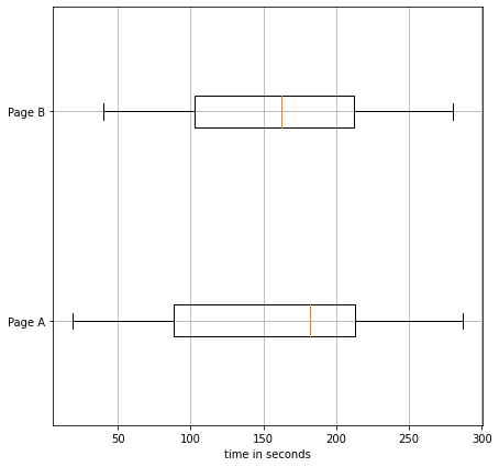
[7]:
fig, ax = plt.subplots(1,1,figsize=(7,7))
ax.boxplot(
    x=[A,B],
    vert=False,
    labels=['Page A','Page B']
)
ax.set_xlabel("time in seconds")
ax.grid()
plt.show()
[8]:
B.mean() - A.mean()
[8]:
5.952380952380963
[9]:
combines = np.hstack((A,B))
combines
[9]:
array([182,  57, 127, 202, 261, 205,  19, 221, 287, 252,  97,  80,  98,
       203,  49, 102, 189, 103, 180,  40,  87, 280, 130, 258, 212, 114,
       192, 258, 162, 162, 280, 200, 142,  47,  46, 217])
[10]:
statistics = []
R = 1000
for i in range(R):
    A_resample = np.random.choice(combines,size=A_size,replace=False)
    B_resample = np.array([i for i in combines if i not in A_resample])

    statistics.append(B_resample.mean() - A_resample.mean())
[11]:
fig, ax = plt.subplots(1,1)
ax.axvline(B.mean() - A.mean(), color='k', label='Observed difference')
ax.hist(statistics,alpha=0.7, label='permutation diff distribution')

ax.legend()
plt.show()
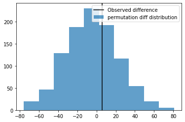
So the Observed Difference is within the range of chance variations, thus is ``not statistically significant``.
Bootstrap#
Resampling with relacement.
Process#
Combine the results from the different groups
Shuffle, then random draw with replacement resample of the same size a group A.
From remaining data, randomly draw with replacement resample of the same size a group B.
Do the same for rest if the groups involved in initial combination.
Calculate the same statistic calculated for original sample, calculate it for new samples, record it. here we have completed one permutation iteration.
Repeat above steps R times, to yield a permutation distribution.
[12]:
np.random.seed(0)

A_size = 15
B_size = 21
total_size = A_size + B_size
A = np.random.randint(low=10, high=300, size=(A_size,))
B = np.random.randint(low=15, high=300, size=(B_size,))

A, B
[12]:
(array([182,  57, 127, 202, 261, 205,  19, 221, 287, 252,  97,  80,  98,
        203,  49]),
 array([102, 189, 103, 180,  40,  87, 280, 130, 258, 212, 114, 192, 258,
        162, 162, 280, 200, 142,  47,  46, 217]))
[13]:
fig, ax = plt.subplots(1,1,figsize=(7,7))
ax.boxplot(
    x=[A,B],
    vert=False,
    labels=['Page A','Page B']
)
ax.set_xlabel("time in seconds")
ax.grid()
plt.show()

[14]:
B.mean() - A.mean()
[14]:
5.952380952380963
[15]:
combines = np.hstack((A,B))
combines
[15]:
array([182,  57, 127, 202, 261, 205,  19, 221, 287, 252,  97,  80,  98,
       203,  49, 102, 189, 103, 180,  40,  87, 280, 130, 258, 212, 114,
       192, 258, 162, 162, 280, 200, 142,  47,  46, 217])
[16]:
statistics = []
R = 1000
for i in range(R):
    A_resample = np.random.choice(combines,size=A_size,replace=True)
    B_resample = np.random.choice(combines,size=B_size,replace=True)

    statistics.append(B_resample.mean() - A_resample.mean())
[17]:
fig, ax = plt.subplots(1,1)
ax.axvline(B.mean() - A.mean(), color='k', label='Observed difference')
ax.hist(statistics,alpha=0.7, label='bootstrap diff distribution')

ax.legend()
plt.show()
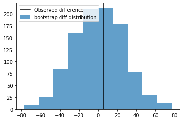
So the Observed Difference is within the range of chance variations, thus is ``not statistically significant``.
Statisitcal Significance#
This is the point where we’ll understanding this topic. Statisitians needs to measure results of an experiment, for that it is required to check whether results of the experiments are more extreme than a random chance might provide. If the result is outside the limits of chance variation then it is said to be statisitcally significant
P Value#
simply observational results are not very precise for statisitcal significance.
It can be understood with the frequency in which the chance model is produces result more extreme than the observed result.measure of statisitcal significance for that
null hypothesisis true.we are talking about a chance model that includes a null hypothesis, the p-value is probability of getting the results within limits or extreme (what are these limits, we’ll see them in next topic).
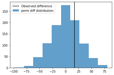
In this case we can calculate p-value from the permutation test we had earlier using permutation distribution differences and observed difference. and get the mean of number of times when the permutation (chance possibility) differences are greater than or equal to observed difference.
[18]:
np.random.seed(0)

A_size = 15
B_size = 21
total_size = A_size + B_size
A = np.random.randint(low=10, high=300, size=(A_size,))
B = np.random.randint(low=10, high=300, size=(B_size,))

combines = np.hstack((A,B))

statistics = []
R = 1000
for i in range(R):
    A_resample = np.random.choice(combines,size=A_size,replace=True)
    B_resample = np.random.choice(combines,size=B_size,replace=True)

    statistics.append(B_resample.mean() - A_resample.mean())

obs_diffs = B.mean() - A.mean()
perm_diffs = np.array(statistics)


print("p-value", np.mean(perm_diffs >= obs_diffs))
p-value 0.257
so the result here is 0.257 or 25.7% times we’ll achieve the same results with chance variation.
[19]:
fig, ax = plt.subplots(1,1)
ax.axvline(obs_diffs, color='k', label='Observed difference')
ax.hist(perm_diffs,alpha=0.7, label='perm diff distribution')

ax.legend()
plt.show()
alpha#
But what is the parameter for unusualness. How do we decide that we have a thershold/ limit for unusualness.
This thershold is specified earlier, like in case of null hypothesis case more extreme than 5%. and this threshold is called alpha.
Typically alpha values(significance level) are 5% or 1%.
probability threshold of ‘unusualness’ that chance results must cross to be statistically significant.
A good question here is given a chance model, what is the probability that results are extreme ?
p-val vs alpha |
interpretation |
|---|---|
Less than 0.01 |
strong evidence against Null Hypothesis, very statistically significant |
0.01 to 0.05 |
Some evidence against Null Hypothesis, statistically significant |
Greater than 0.05 |
Insufficient evidence against Null Hypothesis |
Below example is something I cooked up for this understanding. This may change later.
[20]:
from scipy import stats
np.random.seed(0)

mu, sigma, n_records  = 0, 1, 100
test_results = [-1.5,2.5]

alpha = 0.05 # 5%
data = np.random.normal(loc=mu,scale=sigma,size=n_records)
mean, median, std_dev  = np.mean(data), np.median(data), np.std(data)

#######################################################
# left_bound -- left_side -- right_side -- right_bound
left_bound = -4
left_side = stats.norm.ppf(q=alpha/4)

right_side = -stats.norm.ppf(q=alpha/4)
right_bound = 4

fig = plt.figure(figsize=(10,7))
ax = fig.add_subplot(1,1,1)
sns.distplot(data,bins=20,norm_hist=True)

ax.axvline(mean,label="mean",c='b',lw=4)
ax.axvline(median,label="median",c="r")

for od in test_results:
    pdf_score = stats.norm.pdf(od)
    ax.vlines(od,ymin=0,ymax=pdf_score,color='k',lw=4,alpha=0.7)
    ax.axhline(pdf_score,color='k',ls='--')
    ax.plot(od,pdf_score,'k',marker='o',ms=10,label=f"test-statistc = {od}")
    x_ticks = np.append(ax.get_xticks(), od)
    y_ticks = np.append(ax.get_yticks(), pdf_score)
    ax.set_xticks(x_ticks)
    ax.set_yticks(y_ticks)


ax.axvspan(left_bound, left_side, alpha=0.7, color='grey')
ax.axvspan(right_side, right_bound, alpha=0.7, color='grey')

ax.plot(left_side,alpha/2,'r',marker='o',ms=10)
ax.vlines(left_side,0,alpha/2,color='r',lw=3)


ax.plot(right_side,alpha/2,'r',marker='o',ms=10)
ax.vlines(right_side,0,alpha/2,color='r',lw=3)


ax.axhline(alpha/2,c='r')
y_ticks = np.append(ax.get_yticks(), alpha/2)
ax.set_yticks(y_ticks)

ax.legend()
plt.show()
/home/nishant/.local/lib/python3.9/site-packages/seaborn/distributions.py:2619: FutureWarning: `distplot` is a deprecated function and will be removed in a future version. Please adapt your code to use either `displot` (a figure-level function with similar flexibility) or `histplot` (an axes-level function for histograms).
  warnings.warn(msg, FutureWarning)
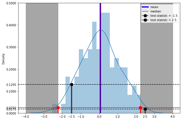
test-statistics |
p-value |
|---|---|
-1.5 |
0.1295 |
2.5 |
0.0175 |
Grey part is showing combined 5% of the data
blue part is showing rest 95% of the data
like test-statisitc -1.5 is in the most population, p-value greater than significance level alpha (p > 0.05)(accept null hypothesis)
and test-statistics 2.5 is in the grey area , p-value less then significance value (p_value < 0.05). making result statisitcally significant against chance variation(reject null hypothesis)
Hypothesis Errors#
Type 1 error |
Type 2 error |
|---|---|
Mistakenly concluding an affect is real(when it is due to chance) |
Mistakenly concluding an affect is due to chance(when it is real) |
Occurs when a researcher rejects the Null Hypothesis when it is true |
Fails to reject the hypothesis when it is false |
False Positive |
False Negative |
Significance Level : probability of commiting a Type 1 error |
Power Of Test : probability of not commiting a Type 2 error |
Statistical Tests#
t-Tests#
t-test generally applies when test statistic would follow a normal distribution.
t-statisitc : standardized version of test statistics.
t-distribution : reference distribution from which observed t-statistic is compared. more details here
Normally estimation for mean and variance of sample is made and test statistics is calculated
if population variance is identified, it is reasonable to consider that test statisics is normally distributed
if population variance is unknown, sample variance is used and test statistics follows t distribution
parent population doesn't need to be normally distributed but population of sample means assumed to be normal.
One Sample#
\begin{align} t-statisitic &= \frac{\bar{x} - \mu_0}{\frac{s}{\sqrt{n}}}\\ \bar{x} &= \text{sample mean}&\\ \mu_0 &= \text{population mean}&\\ s &= \text{sample standard deviation}&\\ n &= \text{sample size}&\\ \text{degree of freedom} &= n - 1&\\ \end{align}
[21]:
from scipy.stats import ttest_1samp,norm,t
[22]:
print(ttest_1samp.__doc__[:250])
Calculate the T-test for the mean of ONE group of scores.

    This is a test for the null hypothesis that the expected value
    (mean) of a sample of independent observations `a` is equal to the given
    population mean, `popmean`.

    Parameters
let significance level is 5% and confidence interval is 95%.
considering it is a two-tailed test then \(\alpha\) = 0.025 (2.5 / 100)
[23]:
alpha = 0.025
generating data
[24]:
mu = 5.0 # population average
sigma = 10 #scale parameter -> std dev -> root(var)
n = 100 #number of observations
rng = np.random.default_rng() #random number generator
[25]:
rvs = norm.rvs(loc=mu, scale=sigma, size=(n,), random_state=0)
assuming that the population is normally distributed and we have a variance.
now lets perform test
[26]:
test_statistic, pvalue = ttest_1samp(rvs,popmean=5.0)
[27]:
test_statistic
[27]:
0.5904283402851683
[28]:
pvalue
[28]:
0.5562489158694683
now if pvalue is greater than \(alpha\), then it is still in confidence level, which means our observation is usual and there is no statistical significance. Null hypothesis is accepted.
else the obsevation is not usual, hence statistical significant result ann Null Hypothesis is rejected.
[29]:
pvalue > alpha
[29]:
True
Null hypothesis is accepted.
Two Samples Unpaired#
This is as straight forward explanation as it can be.
The t-test quantifies the difference between the arithmetic means of the two samples. The p-value quantifies the probability of observing as or more extreme values assuming the null hypothesis, that the samples are drawn from populations with the same population means, is true. A p-value larger than a chosen threshold (e.g. 5% or 1%) indicates that our observation is not so unlikely to have occurred by chance. Therefore, we do not reject the null hypothesis of equal population means. If the p-value is smaller than our threshold, then we have evidence against the null hypothesis of equal population means.
from this doc - https://docs.scipy.org/doc/scipy/reference/generated/scipy.stats.ttest_ind.html
[30]:
from scipy.stats import ttest_ind
Equal sample sizes and variance#
\begin{align} t-statisitic &= \frac{\bar{X_1} - \bar{X_2}}{S_p\sqrt{\frac{2}{n}}}\\ \text{where } S_p &= \sqrt{\frac{S_{X_1}^2 + S_{X_2}^2}{2}}\\ \bar{X_1} &= \text{sample 1 mean}&\\ \bar{X_2} &= \text{sample 2 mean}&\\ S_{X_1} &= \text{sample 1 standard deviation}&\\ S_{X_2} &= \text{sample 2 standard deviation}&\\ n &= \text{sample size}&\\ \text{degree of freedom} &= n - 1&\\ \end{align}
[31]:
rvs1 = norm.rvs(loc=5, scale=10, size=500, random_state=0)
rvs2 = norm.rvs(loc=5, scale=10, size=500, random_state=10)

test_statistic, pvalue = ttest_ind(rvs1, rvs2,equal_var=True)
[32]:
np.corrcoef(rvs1, rvs2)
[32]:
array([[1.       , 0.0190992],
       [0.0190992, 1.       ]])
[33]:
test_statistic
[33]:
-0.9157617644799356
[34]:
pvalue
[34]:
0.3600130785859019
Equal or unequal sample sizes, similar variances#
\begin{align} t-statisitic &= \frac{\bar{X_1} - \bar{X_2}}{S_p\sqrt{\frac{1}{n_1} + \frac{1}{n_2}}}\\ \text{where Pooled variance } S_p &= \sqrt{\frac{(n_1 - 1)S_{X_1}^2 + (n_2 - 1)S_{X_2}^2}{n_1 + n_2 - 2}}\\ \bar{X_1} &= \text{sample 1 mean}&\\ \bar{X_2} &= \text{sample 2 mean}&\\ S_{X_1} &= \text{sample 1 standard deviation}&\\ S_{X_2} &= \text{sample 2 standard deviation}&\\ n_1 &= \text{sample 1 size}&\\ n_2 &= \text{sample 2 size}&\\ \end{align}
equal size data
[35]:
rvs1 = norm.rvs(loc=5, scale=10, size=500, random_state=0)
rvs2 = norm.rvs(loc=5, scale=10, size=500, random_state=10)
Now lets create an unequal size data
[36]:
rvs3 = norm.rvs(loc=5, scale=10, size=100, random_state=10)
test for equal size data
[37]:
ttest_ind(rvs1, rvs2, equal_var=True)
[37]:
Ttest_indResult(statistic=-0.9157617644799356, pvalue=0.3600130785859019)
test for unequal size data
[38]:
ttest_ind(rvs1, rvs3, equal_var=True)
#without trimming the results are not 100% correct, as data1 and data2 are not same size.
[38]:
Ttest_indResult(statistic=-0.9615234228970171, pvalue=0.33667767624405587)
https://en.wikipedia.org/wiki/Welch%27s_t-test
https://www.real-statistics.com/students-t-distribution/problems-data-t-tests/yuen-welchs-test/
[39]:
ttest_ind(rvs1, rvs3, trim=0.2)
[39]:
Ttest_indResult(statistic=-0.9948307819225728, pvalue=0.32049049729267687)
Equal or unequal sample sizes, unequal variances#
\begin{align} t-statisitic &= \frac{\bar{X_1} - \bar{X_2}}{S_{\bar{\Delta}}}\\ \text{where } S_{\bar{\Delta}} &= \sqrt{\frac{S_1^2}{n_1} + \frac{S_2^2}{n_2}}\\ \bar{X_1} &= \text{sample 1 mean}&\\ \bar{X_2} &= \text{sample 2 mean}&\\ S_1 &= \text{sample 1 standard deviation}&\\ S_2 &= \text{sample 2 standard deviation}&\\ n_1 &= \text{sample 1 size}&\\ n_2 &= \text{sample 2 size}&\\ \end{align}
[40]:
rvs1 = norm.rvs(loc=5, scale=10, size=500, random_state=0)
rvs2 = norm.rvs(loc=5, scale=20, size=500, random_state=10)
[41]:
rvs3 = norm.rvs(loc=5, scale=20, size=100, random_state=10)
What if we use the same config of the function
[42]:
ttest_ind(rvs1, rvs2, equal_var=False)
[42]:
Ttest_indResult(statistic=-0.9127612874020155, pvalue=0.3616586927805526)
Now with proper configs
[43]:
ttest_ind(rvs1, rvs2, equal_var=True)
[43]:
Ttest_indResult(statistic=-0.9127612874020156, pvalue=0.3615885407125987)
So if we dont mention that variances are different then this function underestimates pvalue.
Now with unequal sized data
[44]:
ttest_ind(rvs1, rvs3, equal_var=True, trim=0.2)
[44]:
Ttest_indResult(statistic=-1.4564816906088165, pvalue=0.14613596903375511)
Working Example#
[45]:
from sklearn.datasets import load_iris
[46]:
dataset = load_iris()

df = pd.DataFrame(dataset.get('data'),columns=dataset.get('feature_names'))
df['target'] = dataset.get('target')

df
[46]:
| sepal length (cm) | sepal width (cm) | petal length (cm) | petal width (cm) | target | |
|---|---|---|---|---|---|
| 0 | 5.1 | 3.5 | 1.4 | 0.2 | 0 |
| 1 | 4.9 | 3.0 | 1.4 | 0.2 | 0 |
| 2 | 4.7 | 3.2 | 1.3 | 0.2 | 0 |
| 3 | 4.6 | 3.1 | 1.5 | 0.2 | 0 |
| 4 | 5.0 | 3.6 | 1.4 | 0.2 | 0 |
| ... | ... | ... | ... | ... | ... |
| 145 | 6.7 | 3.0 | 5.2 | 2.3 | 2 |
| 146 | 6.3 | 2.5 | 5.0 | 1.9 | 2 |
| 147 | 6.5 | 3.0 | 5.2 | 2.0 | 2 |
| 148 | 6.2 | 3.4 | 5.4 | 2.3 | 2 |
| 149 | 5.9 | 3.0 | 5.1 | 1.8 | 2 |
150 rows × 5 columns
[47]:
X1 = df[df['target'] == 0]['sepal length (cm)'].values #flower 1
X2 = df[df['target'] == 1]['sepal length (cm)'].values #flower 2
[48]:
X1.mean(),np.var(X1)
[48]:
(5.006, 0.12176400000000002)
[49]:
X2.mean(),np.var(X2)
[49]:
(5.936, 0.261104)
Variances are different
Are they independent ?
[50]:
np.corrcoef(X1, X2)
[50]:
array([[ 1.        , -0.08084973],
       [-0.08084973,  1.        ]])
Pearson Correlation Coeff is very low. We can run an independent test.
[51]:
test_statistic, pvalue = ttest_ind(X1, X2, equal_var=False)
test_statistic, pvalue
[51]:
(-10.52098626754911, 3.746742613983842e-17)
[52]:
pvalue > 0.05
[52]:
False
Statistically Significant Result
Two Samples Paired#
[53]:
from scipy.stats import ttest_rel
[54]:
rvs1 = stats.norm.rvs(loc=5, scale=10, size=500, random_state=0)
rvs2 = (stats.norm.rvs(loc=5, scale=10, size=500, random_state=0)+ stats.norm.rvs(scale=0.2, size=500, random_state=10))
[55]:
np.corrcoef(rvs1,rvs2)
[55]:
array([[1.        , 0.99982077],
       [0.99982077, 1.        ]])
Correlation Coeffecient is too high (Close to 1)
[56]:
ttest_rel(rvs1,rvs2)
[56]:
Ttest_relResult(statistic=-0.7326075247954152, pvalue=0.4641418154030663)
Multiple Tests#
Multiple tests notion extends on the thought If you torture the data long enough, it will confess.
Type 1 error - Mistakenly concluding that result is statistically significant.
False discovery rate - In multiple tests, rate of making Type 1 error.
Overfitting - fitting the noise.
Explanation from the book -
lets say that we have 20 predictor variables and 1 target. So if we try to perform hypothesis test on these variables then there is good chance that one predictor will turn out to be (falsely) statistically significant. And it is called Type 1 error.
alpha significance level is 0.05. So, the probability that one will test correctly statistically significant is 0.95. then all 20 will test correctly statistically significant is 0.95 x 0.95 x … x 0.95^20
[57]:
0.95**20
[57]:
0.3584859224085419
Then the probability that at least one predictor will test falsely statistically significant is
1 - (prob all will be significant correctly)
[58]:
1 - 0.95**20
[58]:
0.6415140775914581
64%.. thats something.
Chi-squared(\(\chi^2\)) test (pearson’s)#
A measure of the extent to which some observed data is different from expected value.
Working with categorical distribution and comparison between Observed data and Calculated data.
Goodness of fit test & test for independence
[59]:
import numpy as np
import pandas as pd
Data Sample#
Null Hypothesis : There is no relation between the marital status and educational qualification.
Alternate Hypothesis : There is a significance relation between marital status and educational qualification.
significance level (\(\alpha\)) = 0.05 (95%)
Observed Values
[60]:
obs_data = np.array([
    [18, 36, 21, 9, 6],
    [12, 36, 45, 36, 21],
    [6, 9, 9, 3, 3],
    [3, 9, 9, 6, 3]
])
obs_df = pd.DataFrame(obs_data,columns=['middle school','high school','bachelors','masters','phd'])
obs_df.index = ['never married','married','divorced','widowed']
obs_df
[60]:
| middle school | high school | bachelors | masters | phd | |
|---|---|---|---|---|---|
| never married | 18 | 36 | 21 | 9 | 6 |
| married | 12 | 36 | 45 | 36 | 21 |
| divorced | 6 | 9 | 9 | 3 | 3 |
| widowed | 3 | 9 | 9 | 6 | 3 |
[61]:
cont_table = obs_df.copy()
[62]:
cont_table['columns_total'] = cont_table.values.sum(axis=1)
cont_table
[62]:
| middle school | high school | bachelors | masters | phd | columns_total | |
|---|---|---|---|---|---|---|
| never married | 18 | 36 | 21 | 9 | 6 | 90 |
| married | 12 | 36 | 45 | 36 | 21 | 150 |
| divorced | 6 | 9 | 9 | 3 | 3 | 30 |
| widowed | 3 | 9 | 9 | 6 | 3 | 30 |
[63]:
rows_total = pd.DataFrame(cont_table.values.sum(axis=0).reshape(1,-1), columns=cont_table.columns)
rows_total.index = ['rows_total']

rows_total
[63]:
| middle school | high school | bachelors | masters | phd | columns_total | |
|---|---|---|---|---|---|---|
| rows_total | 39 | 90 | 84 | 54 | 33 | 300 |
[64]:
cont_table = cont_table.append(rows_total)
cont_table
/tmp/ipykernel_3094/882147279.py:1: FutureWarning: The frame.append method is deprecated and will be removed from pandas in a future version. Use pandas.concat instead.
  cont_table = cont_table.append(rows_total)
[64]:
| middle school | high school | bachelors | masters | phd | columns_total | |
|---|---|---|---|---|---|---|
| never married | 18 | 36 | 21 | 9 | 6 | 90 |
| married | 12 | 36 | 45 | 36 | 21 | 150 |
| divorced | 6 | 9 | 9 | 3 | 3 | 30 |
| widowed | 3 | 9 | 9 | 6 | 3 | 30 |
| rows_total | 39 | 90 | 84 | 54 | 33 | 300 |
What I did here ? I calculated rows total and columns total.
Expected Value Calculation -
never married - middle school
\(\frac{90 \times 39}{300} = 11.7\)
married - high school
\(\frac{90 \times 90}{300} = 27\)
[65]:
x = cont_table.values
x
[65]:
array([[ 18,  36,  21,   9,   6,  90],
       [ 12,  36,  45,  36,  21, 150],
       [  6,   9,   9,   3,   3,  30],
       [  3,   9,   9,   6,   3,  30],
       [ 39,  90,  84,  54,  33, 300]])
multiplying rows total and columns total and dividing by complete total.
[66]:
exp_values = (x[:-1,[-1]] @ x[[-1],:-1]) / x[-1,-1]
exp_values
[66]:
array([[11.7, 27. , 25.2, 16.2,  9.9],
       [19.5, 45. , 42. , 27. , 16.5],
       [ 3.9,  9. ,  8.4,  5.4,  3.3],
       [ 3.9,  9. ,  8.4,  5.4,  3.3]])
[67]:
exp_df = pd.DataFrame(
    exp_values,
    columns=['middle school','high school','bachelors','masters','phd']
)
exp_df.index = obs_df.index
exp_df
[67]:
| middle school | high school | bachelors | masters | phd | |
|---|---|---|---|---|---|
| never married | 11.7 | 27.0 | 25.2 | 16.2 | 9.9 |
| married | 19.5 | 45.0 | 42.0 | 27.0 | 16.5 |
| divorced | 3.9 | 9.0 | 8.4 | 5.4 | 3.3 |
| widowed | 3.9 | 9.0 | 8.4 | 5.4 | 3.3 |
[68]:
obs_df
[68]:
| middle school | high school | bachelors | masters | phd | |
|---|---|---|---|---|---|
| never married | 18 | 36 | 21 | 9 | 6 |
| married | 12 | 36 | 45 | 36 | 21 |
| divorced | 6 | 9 | 9 | 3 | 3 |
| widowed | 3 | 9 | 9 | 6 | 3 |
Formula#
\(\text{pearson residual } R = \frac{observed - expected}{\sqrt{expected}}\)
\(\chi^2 = \sum_{i=0}^{r \times c} \frac{(observed - expected)^2} {expected}\)
[69]:
result = np.square(obs_df - exp_df) / exp_df

result
[69]:
| middle school | high school | bachelors | masters | phd | |
|---|---|---|---|---|---|
| never married | 3.392308 | 3.0 | 0.700000 | 3.200000 | 1.536364 |
| married | 2.884615 | 1.8 | 0.214286 | 3.000000 | 1.227273 |
| divorced | 1.130769 | 0.0 | 0.042857 | 1.066667 | 0.027273 |
| widowed | 0.207692 | 0.0 | 0.042857 | 0.066667 | 0.027273 |
[70]:
chi2_value = result.values.sum()
chi2_value
[70]:
23.56689976689977
Degrees of freedom#
\(dof = (r- 1) \times (c - 1)\)
[71]:
r,c = obs_data.shape

dof = (r-1) * (c-1)
dof
[71]:
12
Chi-2 table#
[72]:
alpha = 0.05

chi2_table_value = 21.026
[73]:
chi2_value > chi2_table_value
[73]:
True
Calculate from scipy chi2 cdf
p = 1 - cdf(value, degree_of_freedom)
or use a survival function
p = sf(value, degree_of_freedom)
[74]:
from scipy.stats import chi2
[75]:
chi2.sf(chi2_value,df=dof)
[75]:
0.023281019557072378
Scipy chi2 contingency#
[76]:
from scipy.stats import chi2_contingency
[77]:
chi2_cal, p_value, dof, exp_table = chi2_contingency(observed=obs_data)
[78]:
chi2_cal, p_value, dof
[78]:
(23.56689976689977, 0.023281019557072378, 12)
[79]:
pd.DataFrame(exp_table, columns=obs_df.columns)
[79]:
| middle school | high school | bachelors | masters | phd | |
|---|---|---|---|---|---|
| 0 | 11.7 | 27.0 | 25.2 | 16.2 | 9.9 |
| 1 | 19.5 | 45.0 | 42.0 | 27.0 | 16.5 |
| 2 | 3.9 | 9.0 | 8.4 | 5.4 | 3.3 |
| 3 | 3.9 | 9.0 | 8.4 | 5.4 | 3.3 |
[80]:
alpha, p_value, alpha > p_value
[80]:
(0.05, 0.023281019557072378, True)
thus, rejecting null hypothesis and accepting alternate hypothesis that there is a relation between marital status and education qualification.
ANOVA or Fisher analysis of variance#
If we have multiple groups like A-B-C-D with numeric data, statistical procedure that tests for statistically significant difference amoung the groups is called analysis of variance or ANOVA.
It connects with studies of regression.
One-Way ANOVA#
Pairwise comparison - hyp test(like of means) between two groups amoung multiple groups.
Omnibus test - take all the groups and perform a single hyp test for overall variance among multiple group means.
Sum of Squares (SS) : Deviations from some average value = \(\Sigma{(X- \bar{X})}^2\)
Difference among the groups, called the treatment effect(SSA or SSTR)
Difference within the groups, called error (SSW or SSE)
\(\text{Total Sum of Squares (SSTO) = SSTR + SSE}\)
\(\text{Generally Mean Squares (MS) }=\frac{SS}{degree of freedom}\)
Assumptions
sample is randomly selected from populations and randomly assigned to each of the treatment groups, each observation is thus independent of any other observation - randomness and independence.
Population is considered normally distribution.
\(F-Statistic = \frac{MSTR}{MSE} \sim F_{c-1, n-c}\)
c = number of groups
Source of Variation |
d.f. |
SS |
MS |
F |
P-value |
F-crit |
|---|---|---|---|---|---|---|
Among Groups |
c-1 |
SSTR |
MSTR |
F= MSTR/MSE |
p |
\(F_\alpha\) |
Within Groups |
n-c |
SSE |
MSE |
|||
Total |
n-1 |
SSTO |
[81]:
import numpy as np
Data Sample#
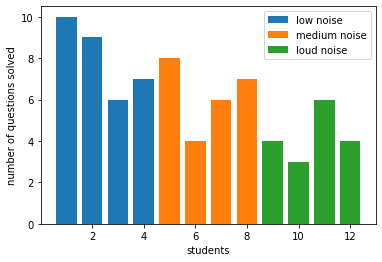
null hypothesis : no significance effect of noise on number of questions solved by students.
alternate hypothesis : there is a significance effect of noise on number of questions solved by students.
[82]:
low_noise = pd.DataFrame(np.array([
    [1, 10],
    [2, 9],
    [3, 6],
    [4, 7]
]),columns=["student","questions"])
low_noise['type'] = 'low noise'

medium_noise = pd.DataFrame(np.array([
    [5, 8],
    [6, 4],
    [7, 6],
    [8, 7]
]),columns=["student","questions"])
medium_noise['type'] = 'medium noise'

loud_noise = pd.DataFrame(np.array([
    [9, 4],
    [10, 3],
    [11, 6],
    [12, 4]
]),columns=["student","questions"])
loud_noise['type'] = 'loud noise'
[83]:
df = pd.concat((low_noise,medium_noise,loud_noise))

df.set_index('type',inplace=True)
[84]:
df
[84]:
| student | questions | |
|---|---|---|
| type | ||
| low noise | 1 | 10 |
| low noise | 2 | 9 |
| low noise | 3 | 6 |
| low noise | 4 | 7 |
| medium noise | 5 | 8 |
| medium noise | 6 | 4 |
| medium noise | 7 | 6 |
| medium noise | 8 | 7 |
| loud noise | 9 | 4 |
| loud noise | 10 | 3 |
| loud noise | 11 | 6 |
| loud noise | 12 | 4 |
[85]:
plt.bar(x=df.loc['low noise']["student"],height=df.loc['low noise']['questions'],label="low noise")
plt.bar(x=df.loc['medium noise']["student"],height=df.loc['medium noise']['questions'], label="medium noise")
plt.bar(x=df.loc['loud noise']["student"],height=df.loc['loud noise']['questions'], label="loud noise")
plt.xlabel("students")
plt.ylabel("number of questions solved")

plt.legend()
plt.show()
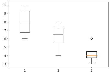
[86]:
plt.boxplot(x=(df.loc['low noise']['questions'], df.loc['medium noise']['questions'],df.loc['loud noise']['questions']))
plt.show()
Calculations#
[87]:
def sum_of_sq(x):
    return np.square(x - x.mean()).sum()
SSTO
[88]:
a = df.loc['low noise'].questions.values
b = df.loc['medium noise'].questions.values
c = df.loc['loud noise'].questions.values
combined = df['questions'].values

SSTO = sum_of_sq(combined)
SSTO
[88]:
51.666666666666664
SSE or SSW
[89]:
SSW = sum_of_sq(a) + sum_of_sq(b) + sum_of_sq(c)
SSW
[89]:
23.5
SSA or SSTR
[90]:
SSA = SSTO - SSW
SSA
[90]:
28.166666666666664
MSA
[91]:
c = 3 #number of groups
MSA = SSA / (c-1)
MSA
[91]:
14.083333333333332
MSW
[92]:
n = combined.shape[0] # total number of samples
MSW = SSW / (n-c)
MSW
[92]:
2.611111111111111
F-Ratio
[93]:
F_value = MSA / MSW
F_value
[93]:
5.3936170212765955
[94]:
from scipy.stats import f
[95]:
f.sf(F_value,dfd=n-c,dfn=c-1)
[95]:
0.02886412420631141
Using Scipy#
[96]:
from scipy.stats import f_oneway
[97]:
f_stat, p_value = f_oneway(
    low_noise.questions,
    medium_noise.questions,
    loud_noise.questions
)
[98]:
f_stat, p_value
[98]:
(5.3936170212765955, 0.02886412420631141)
[99]:
alpha= 0.05

p_value < alpha
[99]:
True
Thus, Rejecting null hypothesis, and accepting alternate hypothesis that there is a significance effect of noise and number of questions solved.
Regression and ANOVA#
[100]:
import statsmodels.api as sm
from statsmodels.stats import anova
import statsmodels.formula.api as smf
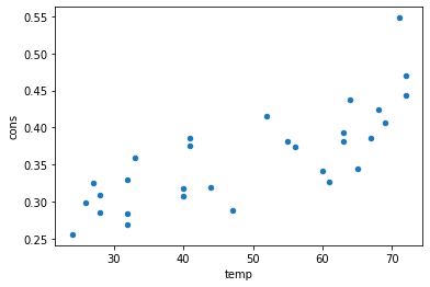
df = sm.datasets.get_rdataset("Icecream", "Ecdat").data
df.head()
[100]:
| cons | income | price | temp | |
|---|---|---|---|---|
| 0 | 0.386 | 78 | 0.270 | 41 |
| 1 | 0.374 | 79 | 0.282 | 56 |
| 2 | 0.393 | 81 | 0.277 | 63 |
| 3 | 0.425 | 80 | 0.280 | 68 |
| 4 | 0.406 | 76 | 0.272 | 69 |
[101]:
df[['cons','temp']].plot(x='temp',y='cons',kind='scatter')
[101]:
<AxesSubplot:xlabel='temp', ylabel='cons'>
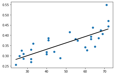
[115]:
model1 = smf.ols('cons ~ temp',data= df )
model1 = model1.fit()
[111]:
preds = model1.predict(df['temp'])
[112]:
plt.scatter(df['temp'],df['cons'])
plt.plot(df['temp'],preds,'k')
[112]:
[<matplotlib.lines.Line2D at 0x7f13e836bd90>]
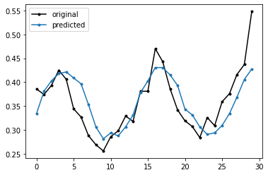
[113]:
plt.plot(df['cons'], 'k.-', label="original")
plt.plot(preds,'.-',label="predicted")
plt.legend()
plt.show()
Null Hypothesis :math:`H_0` : Coefficient of temp is zero
[106]:
print(anova.anova_lm(trainedModel))
            df    sum_sq   mean_sq         F        PR(>F)
temp       1.0  0.075514  0.075514  42.27997  4.789215e-07
Residual  28.0  0.050009  0.001786       NaN           NaN
Null Hypothesis is rejected