Linear Regression#
References#
Intro#
linear regression, a very simple approach for supervised learning. In particular, linear regression is a useful tool for predicting a quantitative response.
In statistics, linear regression is a linear approach to modelling the relationship between a scalar response and one or more explanatory variables (also known as dependent and independent variables).
The case of one explanatory variable is called simple linear regression; for more than one, the process is called multiple linear regression.
                training set
                    |
                    V
            Learning algorithm
                    |
                    V
            +-------------+
test -->    | hypothesis  | --> estimation
            |    / Model  |
            +-------------+
\begin{align*} \text{Hypothesis } h_\theta(x) &= \theta_0 + \theta_1 x \text{, Where Parameters } : \theta_0, \theta_1 \end{align*}
\begin{align*} \text{Cost Function } &: J(\theta_0,\theta_1) = \frac{1}{2m}\sum_{i=1}^{m}(h_\theta{(x^{(i)}) - y^{(i)}})^2\\ \\ \text{Goal} &: {{minimize}\atop{\theta_0,\theta_1}} J(\theta_0,\theta_1) \end{align*}
Generate Data#
[1]:
import pandas as pd
import numpy as np
from sklearn.datasets import make_regression
import matplotlib.pyplot as plt
from mpl_toolkits import mplot3d
import seaborn as sns
[2]:
sample_size = 300
train_size = 0.7 # 70%
X, y = make_regression(n_samples=sample_size, n_features=1, noise=50, random_state=0)
y = y.reshape(-1, 1)
np.random.seed(10)
random_idxs = np.random.permutation(np.arange(0, sample_size))[
: int(np.ceil(sample_size * train_size))
]
X_train, y_train = X[random_idxs], y[random_idxs]
X_test, y_test = np.delete(X, random_idxs).reshape(-1, 1), np.delete(
y, random_idxs
).reshape(-1, 1)
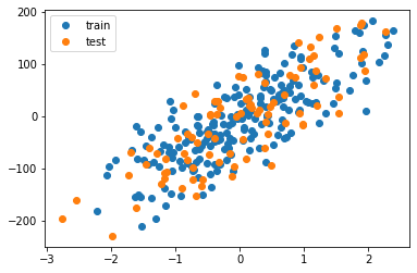
plt.plot(X_train, y_train, "o", label="train")
plt.plot(X_test, y_test, "o", label="test")
plt.legend()
plt.show()
- X = (m,n), wherem = number of samplesn = number of features
Add \(X_0\) (column 0 as 1) for bias in linear regression \begin{align} h_\theta(x) &= \theta_0 X_0 + \theta_1 X_1 \\ \because X_0 &= 1 \\ h_\theta(x) &= \theta_0 + \theta_1 X_1 \\ \end{align}
[3]:
print(X.shape, y.shape)
(300, 1) (300, 1)
[4]:
m, n = X.shape
print("number of columns (features) :", n)
print("number of samples (rows) :", m)
number of columns (features) : 1
number of samples (rows) : 300
[5]:
def add_axis_for_bias(X_i):

    X_i = X_i.copy()
    if len(X_i.shape) == 1:
        X_i = X_i.reshape(-1, 1)

    if False in (X_i[..., 0] == 1):
        return np.hstack(tup=(np.ones(shape=(X_i.shape[0], 1)), X_i))
    else:
        return X_i
Check for bias column(column 0)#
[6]:
arr = np.array(
    [
        [1, 2, 3, 4],
        [1, 6, 7, 8],
        [1, 11, 12, 13],
        [1, 4, 2, 4],
        [1, 5, 2, 1],
        [1, 7, 54, 23],
    ]
)

arr.shape
[6]:
(6, 4)
this means 6 rows and 4 columns
[7]:
False not in (arr[..., 0] == 1)
[7]:
True
[8]:
np.sum(arr), np.sum(arr, axis=0), np.sum(arr, axis=1)
[8]:
(174, array([ 6, 35, 80, 53]), array([10, 22, 37, 11, 9, 85]))
[9]:
np.mean(arr), np.mean(arr, axis=0), np.mean(arr, axis=1)
[9]:
(7.25,
 array([ 1.        ,  5.83333333, 13.33333333,  8.83333333]),
 array([ 2.5 ,  5.5 ,  9.25,  2.75,  2.25, 21.25]))
for us calculation will be done column wise so axis = 0 everywhere
Regression Models Error Evaluation Functions#
Mean Squared Error#
[10]:
def calculate_mse(y_pred, y):
    return np.square(y_pred - y).mean()
Root Mean Squared Error#
[11]:
def calculate_rmse(y_pred, y):
    return np.sqrt(np.square(y_pred - y).mean())
Mean Absolute Error#
[12]:
def calculate_mae(y_pred, y):
    return np.abs(y_pred - y).mean()
Algorithm#
Cost Function#
\begin{align} J(\theta_0,\theta_1) & =\frac{1}{2m}\sum_{i=1}^{m}({h_\theta{(x^{(i)}) - y^{(i)}}})^2 \end{align}
[13]:
def calculate_cost(y_pred, y):
    return np.mean(np.square(y_pred - y)) / 2
Derivative#
\begin{align*} \frac{\partial J(\theta_0,\theta_1)}{\partial \theta} &= \frac{1}{m} \sum_{i=1}^{m}(h_{\theta}(x^{(i)}) - y^{(i)}). x^{(i)} \end{align*}
[14]:
def derivative(X, y, y_pred):
    return np.mean((y_pred - y) * X, axis=0)
Gradient Descent Algorithm#
\begin{align*} \text{repeat until convergence } \{ \\ \theta_j &:= \theta_j - \alpha \frac{\partial}{\partial\theta_j}{J(\theta_0,\theta_1)}\\ \}\text{ for j=0 and j=1 } \\\\ \text{and simultaneously update }\\ temp_0 &:= \theta_0 - \alpha\frac{\partial}{\partial\theta_0}{J(\theta_0,\theta_1)}\\ temp_1 &:= \theta_1 - \alpha\frac{\partial}{\partial\theta_1}{J(\theta_0,\theta_1)}\\ \theta_0 &:= temp_0\\ \theta_1 &:= temp_1 \end{align*}
Final algorithm#
\begin{align*} \text{repeat until convergence }\{\\ \theta_0 &:= \theta_0 - \alpha \frac{1}{m}{\sum_{i=1}^{m}{(h_\theta(x^{(i)}) - y^{(i)})}}\\ \theta_1 &:= \theta_1 - \alpha \frac{1}{m}{\sum_{i=1}^{m}{(h_\theta(x^{(i)}) - y^{(i)})}}.{x^{(i)}}\\ \} \end{align*}
Generate Prediction#
[15]:
def predict(theta, X):
    format_X = add_axis_for_bias(X)

    if format_X.shape[1] == theta.shape[0]:
        y_pred = format_X @ theta  # (m,1) = (m,n) * (n,1)
        return y_pred
    elif format_X.shape[1] == theta.shape[1]:
        y_pred = format_X @ theta.T  # (m,1) = (m,n) * (n,1)
        return y_pred
    else:
        raise ValueError("Shape is not proper.")
Batch Gradient Descent#
[16]:
def linear_regression_bgd(
    X, y, verbose=True, theta_precision=0.001, alpha=0.01, iterations=10000
):
    X = add_axis_for_bias(X)

    # number of features+1 because of theta_0
    m, n = X.shape

    theta_history = []
    cost_history = []

    theta = np.random.rand(1, n) * theta_precision

    for _ in range(iterations):
        # calculate y_pred
        theta_history.append(theta[0])

        y_pred = predict(theta, X)

        # simultaneous operation
        gradient = derivative(X, y, y_pred)

        theta = theta - (alpha * gradient)  # override with new θ

        if np.isnan(np.sum(theta)) or np.isinf(np.sum(theta)):
            print("breaking. found inf or nan.")
            break

        # calculate cost to put in history
        cost = calculate_cost(predict(theta, X), y)

        cost_history.append(cost)

    return theta, np.array(theta_history), np.array(cost_history)
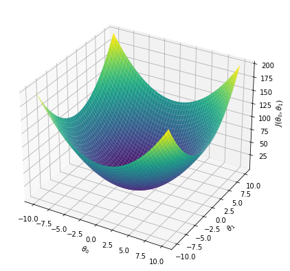
Cost function vs weights \(J(\theta_0, \theta_1)\)#
[17]:
theta0, theta1 = np.meshgrid(np.linspace(-10, 10, 100), np.linspace(-10, 10, 100))
j = theta0**2 + theta1**2

fig = plt.figure(figsize=(7, 7))
ax = plt.axes(projection="3d")

ax.plot_surface(theta0, theta1, j, cmap="viridis")
ax.set_xlabel("$\\theta_0$")
ax.set_ylabel("$\\theta_1$")
ax.set_zlabel("$J(\\theta_0,\\theta_1)$")

plt.show()
Debugging gradient descent#
if learning rate is high, theta value will increase too much and eventually shoot out of the plot.
see an example below.if learning rate is appropriate then value of cost/loss will decrease and eventually flatlines (decrement is too less to matter).
see an example belowwe can try different learning rate like 0.001, 0.003, 0.01, 0.03, 0.1 etc.
Animation Function#
[18]:
from utility import regression_animation
Training with high learning rate#
[19]:
iterations = 600
learning_rate = 2.03

theta, theta_history, cost_history = linear_regression_bgd(
    X_train,
    y_train,
    verbose=True,
    theta_precision=0.001,
    alpha=learning_rate,
    iterations=iterations,
)

regression_animation(
    X_train, y_train, cost_history, theta_history, iterations, interval=10
)
[19]:
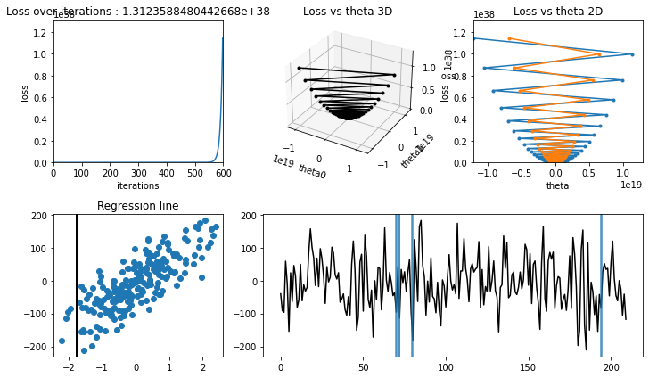
learning rate is high, model couldn’t converge(find minima in loss-theta curve), hence :math:`J(theta_0, theta_1)` increased.
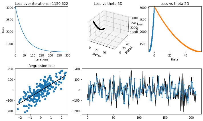
Training with learning rate = 0.01#
[20]:
iterations = 300
learning_rate = 0.01

theta, theta_history, cost_history = linear_regression_bgd(
    X_train,
    y_train,
    verbose=True,
    theta_precision=0.001,
    alpha=learning_rate,
    iterations=iterations,
)

regression_animation(
    X_train, y_train, cost_history, theta_history, iterations, interval=10
)
[20]:
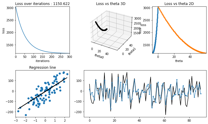
Testing#
[21]:
regression_animation(
    X_test, y_test, cost_history, theta_history, iterations, interval=10
)
[21]:
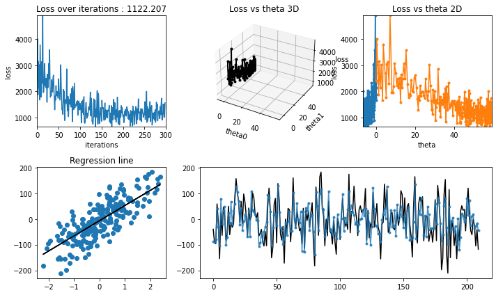
Stochastic gradient Descent#
Stochastic gradient descent (often abbreviated SGD) is an iterative method for optimizing an objective function with suitable smoothness properties (e.g. differentiable or subdifferentiable).
It can be regarded as a stochastic approximation of gradient descent optimization, since it replaces the actual gradient (calculated from the entire data set) by an estimate thereof (calculated from a randomly selected subset of the data).
Especially in high-dimensional optimization problems this reduces the computational burden, achieving faster iterations in trade for a lower convergence rate.
It is
an iterative method
train over random samples of a batch size instead of training on whole dataset
faster convergence on large dataset
[22]:
def linear_regression_sgd(
    X,
    y,
    verbose=True,
    theta_precision=0.001,
    batch_size=30,
    alpha=0.01,
    iterations=10000,
):
    X = add_axis_for_bias(X)

    # number of features+1 because of theta_0
    m, n = X.shape

    theta_history = []
    cost_history = []

    theta = np.random.rand(1, n) * theta_precision

    for iteration in range(iterations):

        theta_history.append(theta[0])

        # creating indices for batches
        indices = np.random.randint(0, m, size=batch_size)

        # creating batch for this iteration
        X_rand = X[indices]
        y_rand = y[indices]

        y_pred = predict(theta, X_rand)

        # simultaneous operation
        gradient = derivative(X_rand, y_rand, y_pred)
        theta = theta - (alpha * gradient)

        if np.isnan(np.sum(theta)) or np.isinf(np.sum(theta)):
            print("breaking. found inf or nan.")
            break

        # calculate cost to put in history
        cost = calculate_cost(predict(theta, X_rand), y_rand)
        cost_history.append(cost)

        # calcualted theta in history
    return theta, np.array(theta_history), np.array(cost_history)
Training for learning rate = 0.01#
[23]:
iterations = 300
learning_rate = 0.01

theta, theta_history, cost_history = linear_regression_sgd(
    X_train,
    y_train,
    verbose=True,
    theta_precision=0.001,
    alpha=learning_rate,
    iterations=iterations,
)

regression_animation(
    X_train, y_train, cost_history, theta_history, iterations, interval=10
)
[23]:
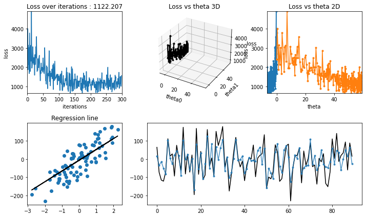
[24]:
regression_animation(
    X_test, y_test, cost_history, theta_history, iterations, interval=10
)
[24]:
Normal Equation (Closed Form)#
normal equation vs gradient descent
Gradient Descent |
Normal Equation |
|---|---|
Need to choose learning rate alpha |
no need to choose alpha |
needs iteration |
doesn’t need iterations |
works well with large number of features ( n large ) |
computation increases for large n |
feature scaling will help in convergence |
no need to do feature scaling |
Derivation#
\begin{align*} & L(\theta) = \frac{1}{n} \sum_{i=0}^{n-1} (\theta^T x - y)^2 \\\\ & \text{where } \vec{x}: (m \times n) \quad \vec{y}: (m \times 1) \quad \vec{\theta}: (n \times 1) , \text{lets take matrix form } & (X \theta - y)^2 = (X \theta - y)^T (X \theta - y) \\\\ & (X \theta - y)^2 = \theta^T X^T X \theta - \theta^T X^T y - y^T X \theta - y^T y \\\\ & \because \theta^T X^T y : (1 \times n)(n \times m)(m \times 1) = (1 \times 1) = \text{scalar value} \\\\ & \text{and } y^T X \theta : (1 \times m)(m \times n)(n \times 1) = (1 \times 1) = \text{scalar value} \\\\ & \text{and } a^T b = b^T a \text{ for scalar value} \\\\ & \therefore (X \theta - y)^2 = \theta^T X^T X \theta - 2 \theta^T X^T y - y^T y \\\\ & \text{to find minima equating dervative of } \theta \text{ to zero} \\\\ & \frac{\delta L}{\delta \theta} = 0 \\\\ & 2 X^T X \theta - 2 X^T y = 0 \\\\ & X^T X \theta = X^T y \\\\ & \theta = (X^T X)^{-1} X^T y \end{align*}
[25]:
def linear_regression_normaleq(X, y):
    X = add_axis_for_bias(X)
    theta = np.linalg.inv(X.T @ X) @ X.T @ y
    return theta
[26]:
theta = linear_regression_normaleq(X_train, y_train)
[27]:
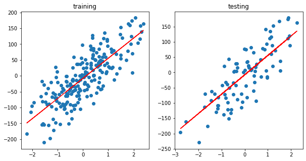
fig, ax = plt.subplots(1, 2, figsize=(10, 5))

y_pred = predict(theta, X_train)

ax[0].scatter(X_train, y_train)
ax[0].plot(X_train, y_pred, c="r")
ax[0].set_title("training")

y_pred = predict(theta, X_test)

ax[1].scatter(X_test, y_test)
ax[1].plot(X_test, y_pred, c="r")
ax[1].set_title("testing")

plt.show()