Basics of Statistics#
[1]:
from scipy import stats
import numpy as np
import matplotlib.pyplot as plt
from matplotlib import style


plt.style.use('seaborn')
Type of data#
Continuous#
Any value within an interval is acceptable. like float, interval
[2]:
cv = np.random.random_sample(10) # continuous values
cv
[2]:
array([0.66031092, 0.65617515, 0.03930539, 0.09361998, 0.85361171,
       0.69670654, 0.91267306, 0.59063556, 0.48679222, 0.64625406])
Discrete#
Only integers are acceptable. countables.
[3]:
dv = np.random.randint(0,10,10) # discrete values
dv
[3]:
array([6, 8, 2, 2, 3, 9, 5, 8, 5, 6])
Categorical#
Ordinal#
Categorical data with explicit ordering. Like encoded in a series
[4]:
np.array([1, 2, 3, 4, 5])
[4]:
array([1, 2, 3, 4, 5])
Nominal#
specific set of values from a category. there is no ordering, counting.
[5]:
np.array([
    'apple',
    'orange',
    'grapes'
])
[5]:
array(['apple', 'orange', 'grapes'], dtype='<U6')
Binary#
only two possible categories, like a switch.
[6]:
np.array([True, False])
[6]:
array([ True, False])
Location Estimates#
mean(average)#
\(\mu=\frac{1}{m}\sum_{i=1}^{m}X^{(i)}\)
[7]:
dv,dv.mean()
[7]:
(array([6, 8, 2, 2, 3, 9, 5, 8, 5, 6]), 5.4)
trimmed mean#
sorted values are trimmed p values from edges,to remove extreme values for mean calculation.
\(\mu = \frac{\sum_{i=p+1}^{m-p} X^{(i)}}{m - 2p}\)
[8]:
p = 2

dv.sort()

dv, dv[p : -p].mean()
[8]:
(array([2, 2, 3, 5, 5, 6, 6, 8, 8, 9]), 5.5)
weighted mean#
mean where weights are associated to the values.
\(\mu_w=\frac{\sum_{i=1}^{m} w^{(i)} X^{(i)}}{\sum_{i=1}^{m}w^{(i)}}\)
[9]:
x = np.random.random_sample(10)
w = np.random.randint(1,4,10)

x, w, (x * w).sum() / w.sum()
[9]:
(array([0.47831889, 0.15173979, 0.65283203, 0.49839894, 0.12887122,
        0.40593656, 0.46486771, 0.03209976, 0.96926736, 0.72582018]),
 array([1, 2, 2, 3, 1, 3, 1, 1, 1, 2]),
 0.4616009083013748)
median#
the value such that one-half of the data lies above and below. (like 50th percentile)
why do we need median? It has less sensitive to data but still what value it can give. median only depends on the data that is located in the center of the sorted array.
so lets take an example of comparing two sets of values of incomes of two regions. if one region has an outlier(very very very rich people). then mean will be a lot different then median. so to compare most common salaries of these two regions, mean will not give best results.
[10]:
x = np.random.random_sample(10)
x
[10]:
array([0.34440759, 0.02302378, 0.26151817, 0.29985192, 0.47751307,
       0.60439014, 0.40955753, 0.27753061, 0.46542145, 0.66317304])
[11]:
sorted(x), np.median(x)
[11]:
([0.023023778580702925,
  0.26151816856942345,
  0.27753060775839367,
  0.29985191612402406,
  0.3444075862196835,
  0.4095575286433396,
  0.46542144991510237,
  0.4775130708375265,
  0.6043901382260869,
  0.6631730366737562],
 0.37698255743151154)
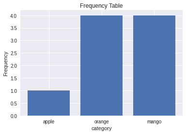
mode#
The most commonly occurring category or value in a data set. It is generally used for categorical dataset and not for numerical dataset.
[12]:
categorical_data = np.array([
    'apple',
    'orange',
    'mango',
    'orange',
    'orange',
    'orange',
    'mango',
    'mango',
    'mango'
])
[13]:
from collections import Counter
[14]:
category_counts = Counter(categorical_data)
category_counts
[14]:
Counter({'apple': 1, 'orange': 4, 'mango': 4})
[15]:
plt.bar(category_counts.keys(),category_counts.values())
plt.title("Frequency Table")
plt.xlabel("category")
plt.ylabel("Frequency")
[15]:
Text(0, 0.5, 'Frequency')
[16]:
category_counts
[16]:
Counter({'apple': 1, 'orange': 4, 'mango': 4})
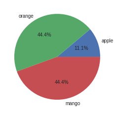
[17]:
plt.pie(category_counts.values(),labels=category_counts.keys(),autopct='%1.1f%%')
plt.show()
[18]:
stats.mode(categorical_data)
[18]:
ModeResult(mode=array(['mango'], dtype='<U6'), count=array([4]))
Variability Estimates#
variability or dispersion to signify whether the data values are tightly clustered or spread out.
variance#
population variance \(\sigma^2 = \frac{\sum{(x - \mu)^2}}{n}\)
sample variance \(s^2 = \frac{\sum{(x - \bar{x})^2}}{n-1}\)
Alternate formula
\begin{align} \Sigma{(x - \mu)}^2 &= \Sigma{(x^2 - 2 x \mu + \mu^2)}\\ &= \Sigma{x^2} - 2 \mu \Sigma{x} + \Sigma \mu^2\\ \because \Sigma{x} = n\mu\\ &= \Sigma{x^2} - 2n \mu^2 + \mu^2 \Sigma{1}\\ &= \Sigma{x^2} - 2n \mu^2 + n\mu^2\\ \Sigma{(x - \mu)}^2 &= \Sigma{x^2} - n \mu^2\\ \sigma^2 &= \frac{\sum{(x - \mu)^2}}{n} = \frac{\Sigma{x^2}}{n} - \mu^2 \end{align}
average of squared difference of each datapoint from dataset’s mean
[21]:
sorted(dv), dv.var(), np.square(dv - dv.mean()).sum() / dv.shape[0] #ddof = 0
[21]:
([2, 2, 3, 5, 5, 6, 6, 8, 8, 9], 5.640000000000001, 5.640000000000001)
[22]:
dv.var(ddof=1), np.square(dv - dv.mean()).sum() / (dv.shape[0] - 1) #ddof = 1
[22]:
(6.2666666666666675, 6.2666666666666675)
degree of freedom(dof)#
degree of freedom describes freedomto vary. The number of observations in data that are free to vary while estimating statistical parameters.
so with possibility that first value could vary and so on 9 values are free to vary but the 10th value is not free to vary because the sum should be 35.
10th value should be a specific number.
degree of freedom = number of observation - number of required relations among the observations
In variance denominator is n-1 not n. But why though? generally n is too large so n or n-1 doesn’t create much difference.
but if we use n as denominator in variance formula, we are underestimating the true value of variance and std deviation in the population. Called biased estimate
and if we use n-1 as denominator then standard deviation becomes an unbiased estimate
deviation#
difference between observed value and estimate of location.
standard deviation#
standard deviation is easier to explain as it is on the same scale as the original data.
population standard deviation \(\sigma = \sqrt \frac{\sum{(x - \mu)^2}}{n}\)
sample standard deviation \(s = \sqrt \frac{\sum{(x - \bar{x})^2}}{n-1}\)
[23]:
## sqrt of variance
dv, dv.std(ddof=0) # ddof = 0
[23]:
(array([2, 2, 3, 5, 5, 6, 6, 8, 8, 9]), 2.3748684174075834)
[24]:
dv, dv.std(ddof=1) # ddof = 1
[24]:
(array([2, 2, 3, 5, 5, 6, 6, 8, 8, 9]), 2.503331114069145)
mean absolute deviation (MAD)#
\(\text{mean absolute deviation} = \frac{\sum{|x - \bar{x}|}}{n}\)
like manhattan norm, l1-norm
[19]:
x = np.random.random_sample(10)
x
[19]:
array([0.75856087, 0.27304572, 0.34091385, 0.65378246, 0.60178779,
       0.61511515, 0.06909667, 0.62935881, 0.59193468, 0.92534561])
[20]:
x, np.abs(x - x.mean()).sum() / x.shape[0]
[20]:
(array([0.75856087, 0.27304572, 0.34091385, 0.65378246, 0.60178779,
        0.61511515, 0.06909667, 0.62935881, 0.59193468, 0.92534561]),
 0.19092524774625713)
range (max - min)#
[25]:
dv, np.ptp(dv)
[25]:
(array([2, 2, 3, 5, 5, 6, 6, 8, 8, 9]), 7)
percentile#
\(Percentile = \frac{rank of value(r_x)}{total values(N)} * 100\)
\(r_x = \frac{Percentile}{100} * {N}\)
[26]:
## a value ,below which lies given the percentage of data points
dv,np.percentile(dv,100, method='lower')
[26]:
(array([2, 2, 3, 5, 5, 6, 6, 8, 8, 9]), 9)
Quartiles#
[27]:
dv, np.percentile(dv,[25,50,75], method='lower')
[27]:
(array([2, 2, 3, 5, 5, 6, 6, 8, 8, 9]), array([3, 5, 6]))
Inter Quartile Range (IQR)#
[28]:
## difference between third quartile Q3 and first quartile Q1

dv, stats.iqr(dv,rng=(25,75), interpolation="lower")
[28]:
(array([2, 2, 3, 5, 5, 6, 6, 8, 8, 9]), 3)
skewness#
majority of the data present on side of the distribution
right skewed |
positive value |
left skewed |
negative value |
unskewed |
zero |
unskewed#
[29]:
np.random.seed(0)
[30]:
ucv = stats.norm(0,1).rvs(10000)
[31]:
ucv.sort()
pdf = stats.norm.pdf(ucv)
[32]:
plt.axvline(ucv.mean(),color='k')
plt.plot(ucv,pdf)
plt.hist(ucv,bins=20,density=True,alpha=0.7)
plt.boxplot(ucv,vert=False)
plt.show()
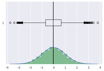
[33]:
## skewness
stats.skew(ucv)
[33]:
0.026634616738395525
right skewed#
[34]:
scv = stats.skewnorm.rvs(4,size=10000)
[35]:
plt.axvline(scv.mean(),color='k')
plt.hist(scv,bins=20,density=True,alpha=0.7)
plt.boxplot(scv,vert=False)
plt.show()
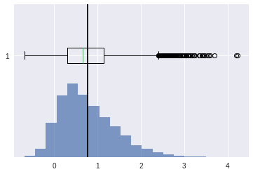
[36]:
## skewness
stats.skew(scv)
[36]:
0.8179623055636133
left skewed#
[37]:
scv = stats.skewnorm.rvs(-4,size=10000)
[38]:
plt.axvline(scv.mean(),color='k')
plt.hist(scv,bins=20,density=True,alpha=0.7)
plt.boxplot(scv,vert=False)
plt.show()
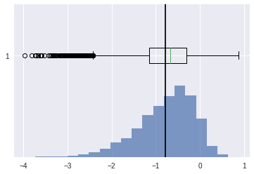
[39]:
## skewness
stats.skew(scv)
[39]:
-0.8325460520764684
Kurtosis#
indicates how much of data is concentrated around mean or shape of the probability distribution.
default Ficsher definition
can be changed to pearson
[40]:
ucv = stats.norm(0,1).rvs(10000)
[41]:
plt.axvline(ucv.mean(),color='k')
plt.hist(ucv,bins=20,density=True,alpha=0.7)
plt.boxplot(ucv,vert=False)
plt.show()
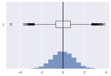
[42]:
## kurtosis
stats.kurtosis(ucv)
[42]:
0.016226092494214583
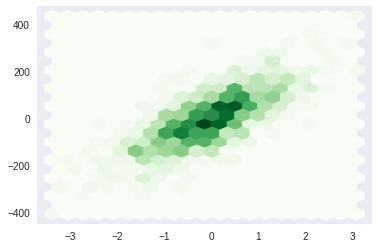
Multi Variate Analysis#
[43]:
from sklearn.datasets import make_regression
[44]:
X, y = make_regression(n_samples=1000,n_features=3)

X.shape, y.shape
[44]:
((1000, 3), (1000,))
hexbin#
[45]:
plt.hexbin(X[...,0], y, gridsize = 20, cmap='Greens')
plt.grid()
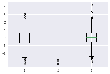
boxplot#
[46]:
plt.boxplot(X)
plt.show()
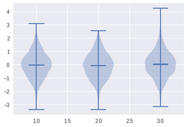
violinplot#
[47]:
plt.violinplot(X,showmeans=True,showextrema=True,showmedians=True)
plt.show()