Support Vector Machine#
References#
https://www.cs.cornell.edu/courses/cs4780/2022fa/lectures/lecturenote09.html
convex optimization docs
https://scikit-learn.org/stable/auto_examples/svm/plot_svm_margin.html
[1]:
import numpy as np
import pandas as pd
import matplotlib.pyplot as plt
import seaborn as sns
from matplotlib import style

plt.style.use("fivethirtyeight")

%matplotlib inline
Assumptions#
Binary Classification y = {-1, 1}
Data is linearly Separable
Concept#

Defining a linear classifier \begin{align*} h(x) = sign(w^T x + b) \end{align*}
binary classification with labels -1 and +1
Typically data is linearly separable and there exist a plane with dimension n - 1 (where n is dimenstion of column space). This plane is defined by
Maximum Margin Hyperplane(Hyperplane is a subspace whose dimension is one less than its ambient space)This mentioned Hyperplane is denoted by \(H\) or \(\mathcal{H}\), is defined by \(\vec{w}\)
As perceptron also creates a hyperplane between the classes to linearly separate them. but it is needed to create a hyperplane that is optimum.
In above diagram we can see 3 hyperplanes. hyperplane 2 and 3 also separates the classes, but the test data point is wrongly classified with hyperplane 2’s scenario. In essence, explaining that plane 2 and 3 are not generalized or optimum solutions.
Maximum Margin Hyperplane#
The plane maximizing the distance to the closest point from both classes
Hyperplane is good if it maximizes the margin (which is minimum distance from both classes)
Margin#

Hyperplane is defined by \(\vec{w}\) as
\begin{align} \mathcal{H} &= \{x | w^T x + b = 0\} \end{align}
\begin{align} \vec{x_p} &= \vec{x} - \vec{d} \\ \because x_p \in H \text{, point on the hyperplane } \therefore w^T x_p + b &= 0 \\ w^T ( \vec{x} - \vec{d} ) + b &= 0\\ \\ \because \text{ d is rescaled vector of w and parallel to it } \therefore \vec{d} &= \alpha \vec{x} \\ \\ w^T ( \vec{x} - \alpha \vec{w} ) + b &= 0\\ \Rightarrow \alpha &= \frac{w^T x + b}{w^T w}\\ \\ \vec{d} &= \frac{w^T x + b}{w^T x} . \vec{x}\\ ||d||_2 &= \sqrt{d^T d} = \sqrt{\alpha^2 w^T w}\\ &= \alpha \sqrt{w^T w} = \frac{w^T x + b}{w^T x} \sqrt{w^T w}\\ ||d||_2 &= \frac{w^T x + b}{\sqrt{w^T w}}\\ ||d||_2 &= \frac{w^T x + b}{||w||_2}\\ \\ \end{align}
Let \(\gamma\) be the minimum distance from the hyperplane and closest point from both classes
\begin{align} \text{margin } \gamma(w, b) = {min\atop{x \in D}} \frac{w^T x + b}{||w||_2} \end{align}
Algorithm#
Now according to the definition of maximum margin classifier
\begin{align} {max\atop{w, b}} \gamma(w, b) \end{align}
But there is a problem with this definition as if we just want to increase the margin it can be anywhere (like \(\infty\) )
This means we need to constraint the hyperplane to be between the classes or the plane of data (necessarily)
Now
\begin{align} {max\atop{w, b}} \gamma(w,b) && \text{ s.t. } && \forall i : y_i (w^T x_i + b) \geq 0 \end{align}
(maximizing the margin to closest points from both classes, such that for all i/samples the classification is correct)
we added constraint to make sure the hyperplane is between the classes, as we know \(y \in \{-1, 1\}\)
if \(w^T x + b = -1\) and correctly classified then \(-1 \times -1 = 1\) and for label 1 as well.
if we move forward with this, then
\begin{align} {max\atop{w, b}} \big[ {min\atop{x \in D}} \frac{|w^T x + b|}{w^ T w} \big] && \mid && \forall i : y_i (w^T x_i + b) \geq 0 \\ \\ \underbrace{{max\atop{w, b}} \frac{1}{w^T w} \big[ {min\atop{x \in D}} |w^T x + b| \big]}_{\text{maximizing the margin}} && \mid && \forall i : \underbrace{y_i (w^T x_i + b) \geq 0}_{\text{correct classifications}} \end{align}
Special Trick#

\begin{align} \text{Hyplane defined as } H &= \{ x : w^T x + b = 0\} \\ \\ {max\atop{w, b}} \frac{1}{w^T w} \big[ {min\atop{x \in D}} |w^T x + b| \big] && \mid && \forall i : y_i (w^T x_i + b) \geq 0 \end{align}
Hyperplane is scale invariant
If we rescale the value of w and b to any positive value (above diagram) then the result is going to be the same (means there is no unique solution)
Hence we can fix values of w and b such that
\begin{align} {\min\atop{x \in D}} | w^T x + b | = 1 \end{align}
\begin{align} \\ \therefore {min\atop{w, b}} w^T w && \mid \forall i: y_i(w^T x_i + b) \geq 0 && && {min\atop{x \in D}} | w^T x + b | = 1 \\ \\ & \Updownarrow \\ \\ {min\atop{w, b}} w^T w && \mid \forall i: y_i(w^T x_i + b) \geq 1 \end{align}
SVM with soft contraints#
what if maximum margin or perfectly separating hyperplane doesn’t exist (ie there will always be one data point misclassified by the algorithm)
We’ll introduce a slack variable
\begin{align*} {min \atop{w,b}} w^T w + c \sum_{i=1}^{n} \xi_i && \forall i : y_i(w^T x_i + b) \geq 1 - \xi_i \\ && \forall i : \xi_i \geq 0 \end{align*}
\begin{align} \xi_i \begin{cases} 1 - y_i (w^T x_i + b) && \text{if } y_i(w^T x_i + b) \lt 1 (\text{misclassifications, 1 x -1 and -1 x 1})\\ \\ 0 && \text{if } y_i(w^T x_i + b) \geq 1 (\text{correctly classified results}) \end{cases} \end{align}
This becomes
\begin{align} {min\atop{w,b}} \underbrace{w^T w}_{l2 regularizer} &+ c \underbrace{\sum \max(1 - y_i (w^T x_i + b), 0)}_{loss}\\ \\ \text{let } c &= \frac{1}{\lambda} \\ \\ L(w, x, b) &= {min \atop{w, b}} \lambda w^T w + \sum \max(1 - y_i (w^T x_i + b), 0) \\ \\ \Rightarrow & {min \atop{w, b}} \frac{1}{n} \sum_{i=1}^{n} \underbrace{l(h_w(x_i), y_i)}_{loss} + \lambda \underbrace{\gamma{(w)}}_{regularizer} \end{align}
Now this is very similar to logistic regression
Gradient Descent#
\begin{align} L(w, x, b) &= {min \atop{w, b}} \lambda w^T w + \sum \max(1 - y_i (w^T x_i + b), 0) \\ \\ L(w, x, b) &= {min \atop{w, b}} \lambda || w ||^2 + \sum \max(1 - y_i (w.x_i + b), 0) \\ \\ \frac{\delta L}{\delta w} &= \begin{cases} 2 \lambda w - y_i x_i & \text{if } y_i(w^T x_i + b) \lt 1 \\ \\ 2 \lambda w & \text{if } y_i(w^T x_i + b) \ge 1 \end{cases} \\ \\ \frac{\delta L}{\delta b} &= - y_i \end{align}
\begin{align} \text{run until convergence } \big\{ \\ \\ w := w - \alpha \frac{\delta L}{\delta w} \\ b := b - \alpha \frac{\delta L}{\delta b} \\ \\ \big\} \end{align}
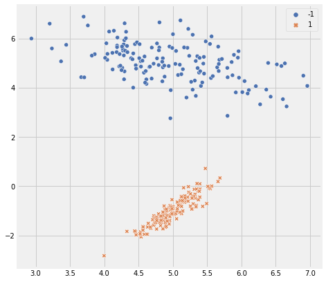
Data Prep#
[11]:
from sklearn.datasets import make_classification
from sklearn import metrics

X, y = make_classification(n_samples=300, n_features=2, n_redundant=0, n_classes=2, shift=2,
                           class_sep=3, n_clusters_per_class=1, random_state=42)

y = np.where(y == 0, 1, -1) # to change classes from 0,1 to -1,1

fig = plt.figure(figsize=(7,7))
ax = fig.add_subplot(1,1,1)
sns.scatterplot(x=X[:,0], y=X[:,1], hue=y, style=y, ax=ax, palette='deep')
plt.show()
Implementation#
[28]:
# np.random.seed(3)

class SVM:
    def __init__(self, n_iter = 100, lambda_param = 0.01, learning_rate = 0.001):
        self.n_iter = n_iter
        self.lambda_param = lambda_param
        self.learning_rate = learning_rate
        self.w = None
        self.b = None
        self.l_loss = None
        self.l_margin = None

    @property
    def margin(self):
        # return 1 / np.linalg.norm(self.w, ord=2)
        return 1 / np.sqrt(np.sum(np.square(model.w)))

    @property
    def loss(self):
        return self.l_loss

    def fit(self, X, y):
        n_samples, n_features = X.shape

        self.w = np.zeros(n_features) #np.random.rand(n_features)
        self.b = 0
        self.l_loss = []
        self.l_margin = []

        for _ in range(self.n_iter):
            for i in range(n_samples):
                if (y[i] * ((self.w @ X[i].T) + self.b)) >= 1:
                    self.w = self.w - ( self.learning_rate * (2 * self.lambda_param * self.w))
                else:
                    self.w = self.w - ( self.learning_rate * (( 2 * self.lambda_param * self.w ) - (y[i] * X[i])))
                    self.b = self.b + ( self.learning_rate * y[i] )

                self.l_loss.append(metrics.hinge_loss(y, self.predict(X)))
                self.l_margin.append(self.margin)


    def predict(self, X):
        return np.sign((self.w @ X.T) + self.b)


    def plot_boundary(self, X, ax=None):
        # np.random.seed(10)

        y_pred = self.predict(X)
        margin = self.margin

        if ax is None:
            fig, ax = plt.subplots(1, 1, figsize=(7, 7))
            ax.set_title("Dicision Boundary - Hyperplane")

        grid_samples = 100

        xx, yy = np.meshgrid(
            np.linspace(X[:, 0].min() - 1 , X[:, 0].max() + 1 , grid_samples),
            np.linspace(X[:, 1].min() - 1 , X[:, 1].max() + 1 , grid_samples)
        )
        mesh = np.c_[xx.ravel(), yy.ravel()]
        mesh_pred = self.predict(mesh)
        zz = mesh_pred.reshape(xx.shape)


        ax.contourf(xx, yy, zz, cmap=plt.cm.coolwarm, alpha=0.2)
        sns.scatterplot(x=X[:, 0], y=X[:, 1], hue=y, style=y, ax=ax, palette='deep')


#         # get the separating hyperplane
#         a = -self.w[0]/self.w[1]
#         xx = np.linspace(X[:, 0].min() - 1, X[:, 0].max() + 1, grid_samples)
#         hyperplane = a * xx - (self.b) / self.w[1]

#         hyperplane_margin_up = hyperplane + a * margin
#         hyperplane_margin_down = hyperplane - a * margin

#         # Plot margin lines
#         ax.plot(xx, hyperplane, 'k-', lw=1)
#         ax.plot(xx, hyperplane_margin_up, 'r--', lw=1)
#         ax.plot(xx, hyperplane_margin_down, 'b--', lw=1)

        ax.legend()

    def plot_loss(self, ax=None):
        if ax is None:
            fig, ax = plt.subplots(1, 1, figsize=(7, 7))
            ax.set_title("Loss over iterations")

        ax.plot(self.loss)


    def plot_margin(self, ax=None):
        if ax is None:
            fig, ax = plt.subplots(1, 1, figsize=(7, 7))
            ax.set_title("Margin over iterations")

        ax.plot(self.l_margin)


    def plot(self, X):
        fig, ax = plt.subplots(1, 3, figsize=(15, 5))

        self.plot_boundary(X, ax=ax[0])
        ax[0].set_title("Dicision Boundary - Hyperplane")

        self.plot_loss(ax=ax[1])
        ax[1].set_title("Loss over iterations")

        self.plot_margin(ax=ax[2])
        ax[2].set_title("Margin over iterations")
[31]:
model = SVM(n_iter=2, lambda_param=0.001, learning_rate=0.01)
model.fit(X, y)
model.plot(X)
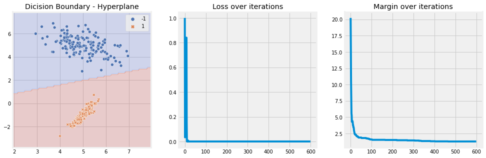
Observations -
Hyplane is perfectly separating the classes.
Loss over iterations is decreasing
Margin over iterations is decreasing
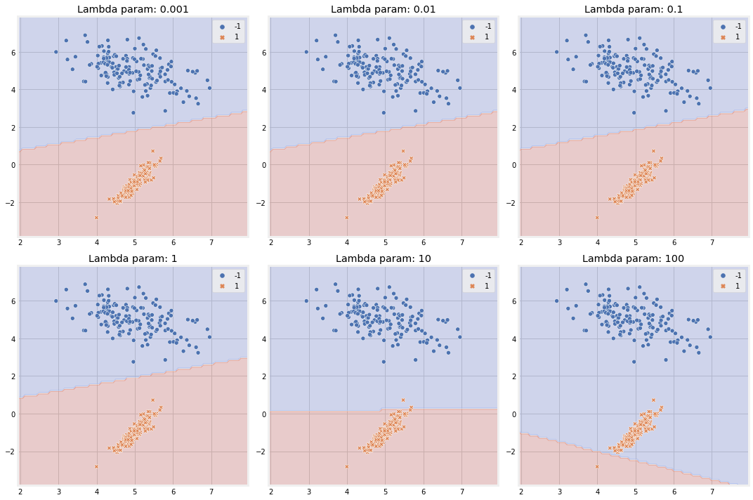
[34]:
fig, ax = plt.subplots(2, 3, figsize=(15, 10))

ax_ = ax.ravel()

for idx, c_ in enumerate([0.001, 0.01, 0.1, 1, 10, 100]):
    model = SVM(n_iter=2, lambda_param=c_, learning_rate=0.001)
    model.fit(X, y)
    model.plot_boundary(X, ax=ax_[idx])
    ax_[idx].set_title(f"Lambda param: {c_}")

plt.tight_layout()
plt.show()